Multiple bounding box detection, Part 3 - fine tuning the backbone network
In the previous posts I focused on preparing the training data:
- Here I data-engineered the full images from the original dataset.
- And here I run the region proposal algorithm to obtain 224x224 regions to be fed to a network that I will train in this post.
Side note: You may wonder why I didn’t choose a more modern network as the backbone of my model, like VisionTransformer or newer architectures. The reason is that I tried to stay true to the original R-CNN architecture, with one exception - they used AlexNet, and I’m using a variation of ResNet, but both are CNNs. Additionally, I’m not very familiar with Vision Transformer architectures yet, so to limit the amount of new information I’d need to take in, I decided to go with something I already know.
Requirements
- Train ResNet-backed feature extractor model.
- Experiment with different sampling strategies.
- Experiment with different loss functions.
The code
No elaborate logic here. The __init__ method constructs image transformation pipelines in accordance with the is_train flag - the pipeline should be different for validation, because for that step no augmentation is needed. Another thing to note is the last line of the transformation pipeline declaration - the one with v2.Normalize - that’s something that ResNet architecture expects. It would work without it too, but the performance could be degraded. As for the __getitem__ method - it’s returning the image name and iou score for debugging. As for the iou score and label - I talked about it in the previous post, but repeating that info here won’t do any harm: a sample is considered to represent the positive class (there’s a crack) if the iou score is > 0.5. That’s in line with the R-CNN paper author’s approach for this phase.
class CrackDataset(Dataset):
    backbone_mean = [0.485, 0.456, 0.406]
    backbone_std = [0.229, 0.224, 0.225]

    def __init__(self, directory: str, image_files: list[str], is_train: bool):
        self.directory = directory
        self.image_files = image_files

        if is_train:
            self.transform = v2.Compose([
                v2.ColorJitter(brightness=0.5),
                v2.RandomHorizontalFlip(p=0.5),
                v2.RandomRotation(180),
                v2.ToImage(),
                v2.ToDtype(torch.float32, scale=True),
                v2.Normalize(mean=self.backbone_mean, std=self.backbone_std)
            ])
        else:
            self.transform = v2.Compose([
                v2.ToImage(),
                v2.ToDtype(torch.float32, scale=True),
                v2.Normalize(mean=self.backbone_mean, std=self.backbone_std)
            ])

    def __len__(self) -> int:
        return len(self.image_files)

    def __getitem__(self, idx: int) -> tuple[torch.Tensor, str, float, int]:
        image_name = self.image_files[idx]
        iou_score, label = CrackDataset.parse_filename(image_name)
        image_path = os.path.join(self.directory, image_name)
        image = Image.open(image_path).convert("RGB")
        image = self.transform(image)

        return image, image_name, iou_score, label

    @staticmethod
    def parse_filename(filename: str) -> tuple[float, int]:
        parts = filename.split(".")
        iou_score = float(parts[2].replace("_", "."))
        label = int(parts[3])

        return iou_score, label
The model itself is quite simple as well. The last layer of ResNet is (fc): Linear(in_features=2048, out_features=1000, bias=True), so there’s no need to flatten anything - I could pass the feature extractor output straight to the ReLU layer. Note the Sigmoid activation at the end - I will talk about it briefly in the training loop section.
At this stage, the feature extractor backbone network is intentionally not frozen. The goal here is to fine-tune the already performant network to the specific problem at hand. In the next post, this retrained network will be reused, this time in a frozen state and a classifier not based on neural networks (an outdated but exciting technique!).
class Resnext50BasedClassifier(nn.Module):
    def __init__(self, input_shape: tuple[int, int, int] = (3, 224, 224)):
        super().__init__()

        self.feature_extractor = models.resnext50_32x4d(weights=ResNeXt50_32X4D_Weights.DEFAULT)
        self.classifier = nn.Sequential(
            nn.ReLU(),
            nn.Linear(self._get_feature_size(input_shape), 1),
            nn.Sigmoid()
        )

    def _get_feature_size(self, shape: tuple[int, int, int]) -> int:
        with torch.no_grad():
            dummy_input = torch.zeros(1, *shape)
            features = self.feature_extractor(dummy_input)

            return features.numel()

    def forward(self, x):
        features = self.feature_extractor(x)
        class_scores = self.classifier(features)

        return class_scores
The next sample is slightly longer than the previous ones. Since I kept running the notebook multiple times, and since the data volume (proposals generated in the second part of this series) is quite big, it made sense to cache the image paths to speed up the file discovery process. Also, you’ll notice that I limited the number of negative samples. I did it to speed up the training. When I allowed the network to go through the whole dataset it was very slow on my RTX3060 graphics card. Apart from that I’m not aiming to train the best possible bounding box detection model, only to learn this particular architecture and have some fun with it. If this was a real world project obviously I would be much more thorough and strict(then again, I would probably have something better than RTX3060 on board ;) ).
def parse_image_metadata(image_name: str):
    parts = image_name.split('.')
    iou_score = float(parts[2].replace('_', '.'))
    label = int(parts[3])

    return iou_score, label


def filter_and_sort_images(image_names: list[str], validation_set: bool) -> list[str]:
    label_0_images = []
    label_1_images = []

    for image_name in image_names:
        iou_score, label = parse_image_metadata(image_name)

        if label == 1:
            label_1_images.append(image_name)
        elif label == 0:
            label_0_images.append((image_name, iou_score))

    set_size = 800 if not validation_set else 200
    label_0_images_sorted = [img for img, _ in sorted(label_0_images, key=lambda x: x[1], reverse=True)[:set_size]]
    filtered_images = label_1_images + label_0_images_sorted

    return filtered_images


def get_image_paths_from_file(file_path: str, images_dir: str, validation_set: bool) -> list[str]:
    if os.path.exists(file_path):
        with open(file_path, 'r') as f:
            print(f"Loading image paths from {file_path}")

            image_paths = json.load(f)
    else:
        print(f"{file_path} not found. Reading image paths from directory.")

        image_paths = [f for f in os.listdir(images_dir) if os.path.isfile(os.path.join(images_dir, f))]

        with open(file_path, 'w') as f:
            json.dump(image_paths, f)

    filtered_images = filter_and_sort_images(image_paths, validation_set)

    return filtered_images


def get_loaders() -> tuple[DataLoader, DataLoader]:
    train_images_dir = DATASETS_PATH / "train"
    valid_images_dir = DATASETS_PATH / "valid"
    train_paths_file = DATASETS_PATH / "train_image_paths.json"
    valid_paths_file = DATASETS_PATH / "valid_image_paths.json"
    train_images_paths = get_image_paths_from_file(train_paths_file, train_images_dir, validation_set=False)

    print(f"Finished reading train images. Total: {len(train_images_paths)} images.")

    valid_images_paths = get_image_paths_from_file(valid_paths_file, valid_images_dir, validation_set=True)

    print(f"Finished reading valid images. Total: {len(valid_images_paths)} images.")

    train_dataset = CrackDataset(train_images_dir, train_images_paths, is_train=True)
    valid_dataset = CrackDataset(valid_images_dir, valid_images_paths, is_train=False)
    train_dataloader = DataLoader(train_dataset, batch_size=BATCH_SIZE, shuffle=True)
    valid_dataloader = DataLoader(valid_dataset, batch_size=BATCH_SIZE)

    return train_dataloader, valid_dataloader
And finally, below you’ll find the training loop. It’s easy to spot that I decided to use the BCELoss instead of the BCEWithLogitsLoss (that’s why I’m using the Sigmoid activation in the classifier module). I chose one over the other because of a few factors:
- I didn’t need to use raw logits anywhere else.
- It’s easier on the testing phase - you just input the data into the model without the need to apply sigmoid on prediction results to obtain class probabilities.
- Vanishing gradients are not an issue here.
I’m gathering the history entries in order to be able to create pretty plots after the training is done.
device = torch.device("cuda" if torch.cuda.is_available() else "cpu")
model = Resnext50BasedClassifier()
criterion = torch.nn.BCELoss()
optimizer = optim.Adam(model.parameters(), lr=0.001)
early_stopping = EarlyStopping(patience=3, verbose=True)
train_loader, valid_loader = get_loaders()

model.to(device)

history = {
    "train_loss": [],
    "train_accuracy": [],
    "val_loss": [],
    "val_accuracy": []
}

for epoch in range(NUM_EPOCHS):
    model.train()

    running_loss = 0.0
    correct_train = 0
    total_train = 0
    epoch_progress = tqdm(train_loader, desc=f"Epoch {epoch+1}/{NUM_EPOCHS} [Training]", unit="batch")

    for images, names, scores, labels in epoch_progress:
        images, labels = images.to(device), labels.float().to(device)

        optimizer.zero_grad()

        outputs = model(images).squeeze()
        predictions = (outputs >= 0.5).float()
        correct_train += (predictions == labels).sum().item()
        total_train += labels.size(0)

        loss = criterion(outputs, labels)
        loss.backward()
        optimizer.step()

        running_loss += loss.item() * images.size(0)

        epoch_progress.set_postfix(
            loss=running_loss / total_train,
            accuracy=100.0 * correct_train / total_train
        )

    train_loss = running_loss / len(train_loader.dataset)
    train_accuracy = 100.0 * correct_train / total_train

    history["train_loss"].append(train_loss)
    history["train_accuracy"].append(train_accuracy)
    print(f"Training Loss: {train_loss:.4f}, Training Accuracy: {train_accuracy:.2f}%")
    model.eval()

    val_loss = 0.0
    correct_val = 0
    total_val = 0

    with torch.no_grad():
        valid_progress = tqdm(valid_loader, desc=f"Epoch {epoch+1}/{NUM_EPOCHS} [Validation]", unit="batch")

        for valid_images, valid_names, valid_scores, valid_labels in valid_progress:
            valid_images, valid_labels = valid_images.to(device), valid_labels.float().to(device)
            outputs = model(valid_images).squeeze()
            predictions = (outputs >= 0.5).float()
            correct_val += (predictions == valid_labels).sum().item()
            total_val += valid_labels.size(0)

            loss = criterion(outputs, valid_labels)
            val_loss += loss.item() * valid_images.size(0)

    val_loss /= len(valid_loader.dataset)
    val_accuracy = 100.0 * correct_val / total_val

    history["val_loss"].append(val_loss)
    history["val_accuracy"].append(val_accuracy)
    print(f"Validation Loss: {val_loss:.4f}, Validation Accuracy: {val_accuracy:.2f}%")
    early_stopping(val_loss, model, SAVE_PATH)

    if early_stopping.early_stop:
        print("Early stopping")
        break
When the model is done training, it’s time for testing. First let’s generate the classification report to see how well it does with the two categories it was supposed to distinguish.
              precision    recall  f1-score   support

    No crack       0.86      0.87      0.86     37111
       Crack       0.67      0.65      0.66     15337

    accuracy                           0.80     52448
   macro avg       0.76      0.76      0.76     52448
weighted avg       0.80      0.80      0.80     52448
The model is not very good - better than random chance in crack detection, but still far from stellar. I didn’t expect great results because of the nature of the problem I chose. To explain, I need to get a bit metaphysical here.
The original R-CNN network was trained on images of people, cars, animals - objects we see daily. This version, however, was retrained on a dataset full of cracks, and this dataset possesses a trait the original one lacked: self-resemblance.
What I mean by this is that if you take a small region of an image containing part of a crack, it still looks like a crack on its own. In contrast, if you take a region of an image of a person - say, a leg, half a face, or part of a torso - it may have some human-like traits, but it doesn’t resemble a complete human.
My hypothesis is that for problems characterized by this self-resemblance trait, precision and recall will tend to underperform. If I’m mistaken, so be it - I’m here to learn and uncovering how the described problem can be solved better will be a great adventure.
But coming back to the classification report: the model performs significantly better at identifying non-crack regions compared to crack regions. This disparity is evident from the higher precision, recall, and F1-score for the “No Crack” class. The “Crack” class shows lower values across all metrics, indicating challenges in accurately identifying cracks. To clearly interpret the numbers:
- When the model predicts a crack, it is correct 67% of the time.
- Recall value shows that the model correctly identified 65% of all actual cracks in the dataset. The remaining 35% of true cracks were missed (false negatives).
For this particular problem it would be best if the recall value for the “Crack” class was higher. Translating to a real-world scenario: imagine a production line in a tile factory with cameras above it. When a new tile comes it, the cameras take photos of it. They are sent to our crack detection system to make sure the company doesn’t sell damaged products. What it means is that we want to detect the maximum number of damaged tiles, even at the expense of reporting some false positives - that’s what optimizing for recall will do. In the following steps I will try to find a way to bump up that numbers, at least slightly. When I obtain a model that does better than this one, I’ll move on to describing the final steps.
For the next iteration of my solution I used class weighing. For that I had to add this method to the dataset class:
    def get_labels(self) -> list[int]:
        """Quickly extract labels without loading images or applying transformations - for the sampler."""
        return [CrackDataset.parse_filename(f)[1] for f in self.image_files]
…and this is the code I added to the get_loaders function:
    train_dataset = CrackDataset(train_images_dir, train_images_paths, is_train=True)
    valid_dataset = CrackDataset(valid_images_dir, valid_images_paths, is_train=False)
    labels = train_dataset.get_labels()
    class_weights = {0: 1, 1: 2}
    sample_weights = [class_weights[label] for label in labels]
    train_sampler = WeightedRandomSampler(weights=sample_weights, num_samples=len(sample_weights), replacement=True)
    train_dataloader = DataLoader(train_dataset, batch_size=BATCH_SIZE, sampler=train_sampler)
    valid_dataloader = DataLoader(valid_dataset, batch_size=BATCH_SIZE)
As you can see, I’m adding more weight to the “crack” class. With conjunction with the replacement=True parameter this means that the “crack” class instances will be selected more often and that a single instance can be selected more than once in an epoch. Assigning a higher weight to an underrepresented class is a common way of improving models performance, let’s see what it did for this particular problem.
              precision    recall  f1-score   support

    No crack       0.89      0.78      0.83     37111
       Crack       0.58      0.76      0.66     15337
Those changes resulted in an interesting improvement to the recall value. It seems that now the model can detect more cracks! However, its precision dropped. Effectively, or at least judging by the f1-score, we’re almost in the same place for the positive class detection but the performance dropped slightly for the negative class (0.78 VS 0.87 recall value in the previous iteration). However, as stated in the previous paragraph, we’re optimizing for the recall, so this direction is the right one. Let’s see if the upcoming changes will bump up the precision metric value for the positive class while keeping recall at the same (decent) level.
Earlier, I mentioned the self-resemblance problem. I don’t have a clear solution for it when using a pretrained network like the ResNet I’m working with in this post. However, I decided to experiment with lowering the IoU threshold as a potential workaround.
My rationale was that the model’s recall is suboptimal because it often gets confused by images that resemble cracks but are labeled as the negative class. Since self-resemblance is present independently of scale, smaller image patches showing parts of cracks might still confuse the model. However, I hope this confusion will be less pronounced, making the lower IoU threshold beneficial.
That said, there’s a trade-off. This adjustment could impair the bounding box detector’s ability to produce well-fitting bounding boxes. The original R-CNN paper justifies the choice of a .5 IoU threshold for this reason. If this happens, I’ll revisit the approach and explore other ways to address the self-resemblance problem while returning to a higher IoU threshold.
These are the classification results for a model trained with a lowered IoU threshold:
              precision    recall  f1-score   support

    No crack       0.84      0.78      0.81     39615
       Crack       0.70      0.78      0.74     26757
At this point I decided to train one more model to see what effect would sampling without replacement have on the model’s performance:
              precision    recall  f1-score   support

    No crack       0.83      0.82      0.82     39615
       Crack       0.73      0.75      0.74     26757
The recall dropped slightly but the precision went up. Depending on the trade-offs that the virtual client is willing to accept I could have picked one of these models and move to the next topic. However, after training these models I thought about using a different loss function - the sigmoid_focal_loss from the torchvision.ops module.
The BCELoss is straightforward (the below is its formula with the default mean reduction):
It penalizes the incorrect predictions based on their confidence, treating all misclassifications equally. It’s good for balanced datasets, and even for the imbalanced ones (like the one I’m using) a lot can be done to improve its workings with class weights (as you saw). However, there’s another loss function which is smarter: sigmoid focal loss function. Here’s its formula when mean reduction is used:
\[\begin{aligned} \text{Focal Loss} = - \frac{1}{N} \sum_{i=1}^{N} \alpha_t \cdot (1 - p_t)^\gamma \cdot BCE Loss_i \end{aligned}\]Where \(p_t\) is defined as (and \(p=\sigma(inputs)\) - i.e., the sigmoid of the raw model outputs):
\[\begin{aligned} p_t = \begin{cases} p & \text{if } y = 1 \\ 1 - p & \text{if } y = 0 \end{cases} \end{aligned}\]The \((1 - p_t)^\gamma\) term is what they call (page 3) a modulating factor. To use the author’s original words: “When an example is misclassified and \(p_t\) is small, the modulating factor is near 1 and the loss is unaffected. As \(p_t \rightarrow 1\), the factor goes to \(0\) and the loss for well-classified examples is down-weighted.” - the loss contribution from easy examples is reduced.
As for the \(\alpha_t\) - it is the weighting factor for class imbalance:
\[\begin{aligned} \alpha_t = \begin{cases} \alpha & \text{if } y = 1 \\ 1 - \alpha & \text{if } y = 0 \end{cases} \end{aligned}\]Translating \(\alpha_t\) to the code that you’ll find in pytorch docs for the sigmoid_focal_loss function, it’s this statement:
alpha_t = alpha * targets + (1 - alpha) * (1 - targets)
Translating it back to mathematical terms (where’s the if-else, goddammit?!), when targets == 1:
\[\begin{aligned} (1 - targets) = 0 \end{aligned}\] \[\begin{aligned} \alpha_t = \alpha \cdot 1 + (1 - \alpha) \cdot 0 = \alpha \end{aligned}\]And when targets == 0:
\[\begin{aligned} (1 - targets) = 1 \end{aligned}\] \[\begin{aligned} \alpha_t = \alpha \cdot 0 + (1 - \alpha) \cdot 1 = 1 - \alpha \end{aligned}\]To give an example using numbers:
\[\begin{aligned} \mathbf{\alpha} = \alpha \cdot \begin{bmatrix} 1 \\ 0 \end{bmatrix} + (1 - 0.25) * (1 - \begin{bmatrix} 1 \\ 0 \end{bmatrix}) = \begin{bmatrix} 0.25 \\ 0.75 \end{bmatrix} \end{aligned}\]I don’t know about you, but this was very counterintuitive for me at first glance. The sigmoid_focal_loss function was supposed to emphasize the loss effect of the underrepresented class, and that numerical example clearly shows that the overrepresented class gets a higher weight.
Although I couldn’t find anything in the cited work and ChatGPT started talking nonsense, I think I eventually came up with the right intuition. The key lies in relating the \(\alpha_t\) to the modulating factor. The later would be very small for very easy examples and very big for hard examples. In general, this is something good but could result in underrepresented samples dominating the loss too much, and therefore a small adjustment is applied. I really hope I got this one right :)
With that explained let’s look at the classification report for a model trained with the sigmoid_focal_loss function with \(\alpha\) and \(\gamma\) parameters set with the default values (btw. the model definition had to be changed slightly - since the loss function itself applies the torch.sigmoid operation, there was no need to use the Sigmoid activation directly in the model - because of that it now returns raw logits):
outputs = model(images).squeeze()
probabilities = torch.sigmoid(outputs)
predictions = (probabilities >= .5).float()
              precision    recall  f1-score   support

    No crack       0.77      0.98      0.86     37111
       Crack       0.83      0.28      0.42     15337
That’s a very bad result, isn’t it? The model is now able to find only 28% of all the crack images. I did a few runs with different \(\alpha\) and \(\gamma\) values, but eventually I gave up. Nothing I did could make the model’s recall go back to the 70-80% level obtained previously. However, on one of my last tries I set \(\alpha = -1\). As visible in the loss function source code, with a value below zero \(\alpha\) is ignored and the loss function becomes an interaction between the modulating factor and the cross entropy term. Guess what? It actually helped in maximizing the recall at the expense of precision going down.
              precision    recall  f1-score   support

    No crack       0.84      0.81      0.82     39615
       Crack       0.73      0.77      0.75     26757
Side note: you might have noticed the support value changes between the two reports. It happened because the IoU threshold was lowered. The specific reason for why the number of “Crack” instances grew is that with a lower threshold, more samples are considered cracks, which is kind of obvious. However, the number of “No crack” instances also grew slightly, so why is that? Look at the filter_and_sort_images function. It takes 10 images from each group of IoU ranges. Let’s consider the top group - \([.35, .5)\). It might have happened that there was a smaller (than 10) number of images in this group, but now these images are considered to be members of the positive category. However, in the lower groups there were usually 10 images. So lowering of the IoU threshold had a side effect of including more “No crack” images because there was just more images without cracks in the lower IoU groups.
Now we end up with two decent models - one with 70% / 78% precision / recall level and the last one that got 73% / 77% precision / recall level for the positice class.
Another side note: I retrained both variations to make sure the numbers are not obtained by chance, and, as you might have guessed - they’re not. That’s the thing with transfer learning. The initial model is already pretty good, so what changes most from epoch to epoch are the added layers. However, since they rely heavily on the features extracted earlier, on each training run they will converge to almost the same numbers.
I also wanted to share the accuracy and loss plots and comment on them. On the left you’ll see the plots for the first model (the one with 70% / 78% precision / recall values), and on the right ones for the last one:

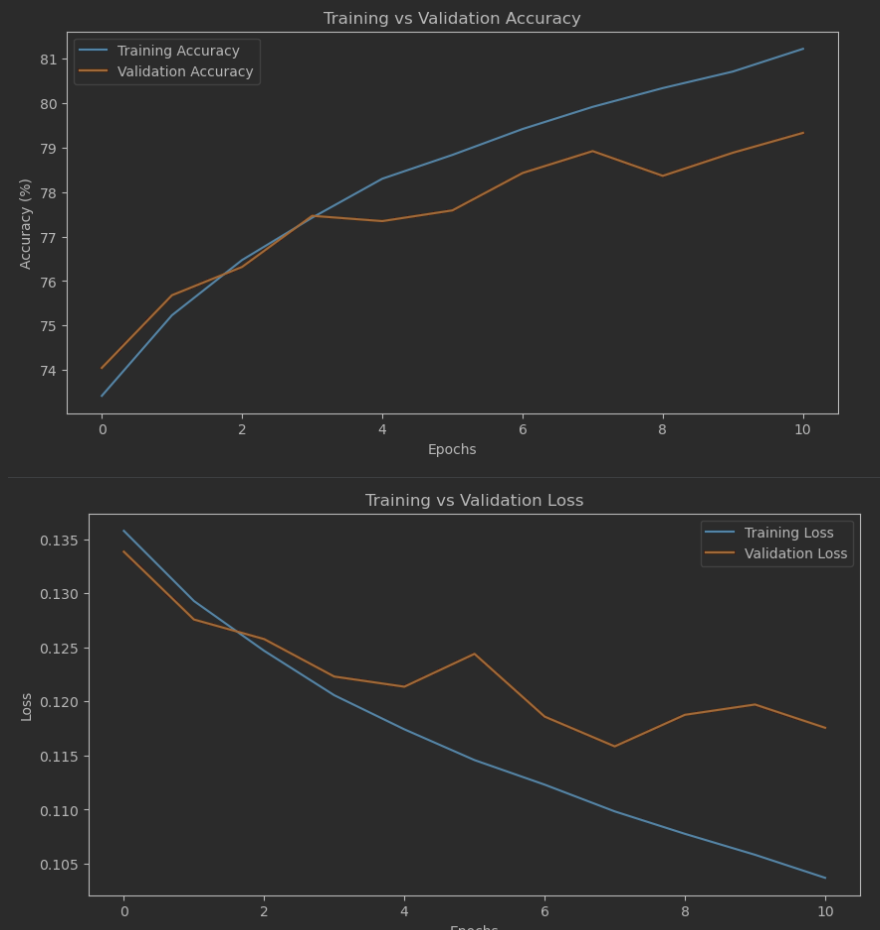
The specific numbers are less interesting than the shapes of the curves. In the first variation, there are clear signs of overtraining - notice how far apart the curves are from one another. In contrast, for the second variation, the gap between the curves is much smaller. This is the second reason why I’ve decided to use the second variation in the next steps.
Summary and next steps
This project was a lot of fun, especially the experimentation with the loss function. What surprised me the most was how well it worked, despite being designed for larger problems - at least, according to what I found on the internet. I half-expected it wouldn’t improve the results or might even make them slightly worse. This is a common outcome when more complex mechanisms end up underperforming compared to simpler ones.
As I mentioned at the beginning of this series, I’m not striving for perfection. That’s why I decided to stop where I did. The results are far from perfect, and perhaps using a more modern backbone network architecture could improve them. However, as I said earlier, perfection isn’t the goal here.
Next up: I’ll drop the neural net classifier and try to perform the second step described in the R-CNN work which is training an SVM classifier.