Multiple bounding box detection, Part 1 - data preparation
This post is the first in a series that I’ve long planned to write. At the time of writing, I don’t know how many parts there will be or their specific topics, but what I can be sure of is that I will attempt to implement major components of R-CNN, Fast(er) R-CNN, and Mask R-CNN.
One important remark - this is a learning experience for me, this whole blog is. I suppose that I won’t be able to maximize the performance of my models, but that’s not the goal of this series. I’m saying this in the beginning, just so that remember it after I come back to these posts after long time, or if someone wonders “why didn’t he use technique X - that would make the accuracy skyrocket over 100%” ;)
The initial idea was to train my networks using this kaggle dataset, and then test them on something else. However, given how different the other dataset is, I may instead train on a subset of the first one and test on the remaining portion. We’ll see how it goes :)
This part will focus on performing some data engineering steps to prepare the data.
Requirements
The goal here is to prepare a list of bounding boxes for the neural networks to train on. The kaggle dataset contains segmentation masks, but it doesn’t contain bounding box coordinates, so the requirement is to calculate those from the segmentation masks. The thing is, some of them are of bad quality. Take a look at two examples of such images:
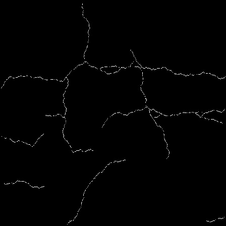
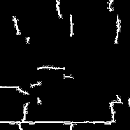
If you look closely at the first image, you’ll notice it consists of clusters of white pixels, often not connected to each other. This means that if I were to use this mask directly, it would detect tens of separate bounding boxes. The other example presents a different issue. It’s hard to describe exactly what’s visible - there are some strange artifacts surrounding the actual correct masks, which will also need to be addressed.
To sum up, the requirement I came up with for preprocessing the images to obtain bounding boxes is to do it in a way that limits the number of bounding boxes when small, disconnected clusters of pixels are detected.
The code
Data engineering
There are very few necessary imports that need to be present.
import os
import cv2
import json
import numpy as np
Apart from that some initial variables need to be set up for the later code.
train_dir = os.path.join("data", "train")
valid_dir = os.path.join("data", "valid")
images_dir_train = os.path.join(train_dir, "images")
images_dir_valid = os.path.join(valid_dir, "images")
masks_dir_train = os.path.join(train_dir, "masks")
masks_dir_valid = os.path.join(valid_dir, "masks")
For storing the data about the images I again choose the COCO format. The below function returns a template dictionary to be filled in and extended in the code presented next.
def get_coco_tpl() -> dict:
    return {
        "images": [],
        "annotations": [],
        "categories": [{
            "id": 1,
            "name": "crack",
            "supercategory": "defect"
        }]
    }
The function below satisfies the requirement mentioned in the previous section. In each iteration, it takes a box from the top of the bboxes list and then iterates over the remaining ones. At each step, it checks if the current bounding box lies in proximity to another one, regulated by the threshold parameter. If they are close enough, it builds a new bounding box that encompasses both of them. This new bounding box replaces the original one and is used in the next iteration for comparison with other bounding boxes in the list. Through this process, larger and larger bounding boxes are created, reducing the final count to a sufficiently small number.
def merge_adjacent_bboxes(bboxes: list[list[int]], threshold: int = 10) -> list[list[int]]:
    merged_bboxes = []

    while bboxes:
        current_bbox = bboxes.pop(0)
        merged = True

        while merged:
            merged = False

            for i, bbox in enumerate(bboxes):
                if (current_bbox[0] - threshold < bbox[0] + bbox[2] and
                    current_bbox[0] + current_bbox[2] + threshold > bbox[0] and
                    current_bbox[1] - threshold < bbox[1] + bbox[3] and
                    current_bbox[1] + current_bbox[3] + threshold > bbox[1]):

                    x_min = min(current_bbox[0], bbox[0])
                    y_min = min(current_bbox[1], bbox[1])
                    x_max = max(current_bbox[0] + current_bbox[2], bbox[0] + bbox[2])
                    y_max = max(current_bbox[1] + current_bbox[3], bbox[1] + bbox[3])
                    current_bbox = [x_min, y_min, x_max - x_min, y_max - y_min]
                    bboxes.pop(i)
                    merged = True
                    break

        merged_bboxes.append(current_bbox)

    return merged_bboxes
The above function is then used in the below one:
def find_boxes(images_dir: str, masks_dir: str, coco_format: dict, closing_kernel_size: int = 15) -> None:
    annotation_id = 1
    image_id_mapping = {}
    kernel = np.ones((closing_kernel_size, closing_kernel_size), np.uint8)

    for mask_filename in os.listdir(masks_dir):
        image_id = os.path.splitext(mask_filename)[0]

        if "cracktree" in image_id.lower():
            continue

        mask_path = os.path.join(masks_dir, mask_filename)
        image_path = os.path.join(images_dir, f"{image_id}.jpg")

        if not os.path.exists(image_path):
            continue

        image_id_mapping[image_id] = len(image_id_mapping) + 1
        mask = cv2.imread(mask_path, cv2.IMREAD_GRAYSCALE)

        if mask is None or np.sum(mask) == 0:
            annotation_entry = {
                "id": annotation_id,
                "image_id": image_id_mapping[image_id],
                "category_id": 1,
                "bbox": [],
                "area": 0,
                "segmentation": [],
                "iscrowd": 0,
                "label": f"no crack {annotation_id}"
            }
            coco_format["annotations"].append(annotation_entry)
            annotation_id += 1

        closed_mask = cv2.morphologyEx(mask, cv2.MORPH_CLOSE, kernel)
        _, binary_image = cv2.threshold(closed_mask, 127, 255, cv2.THRESH_BINARY)
        num_labels, labels, stats, centroids = cv2.connectedComponentsWithStats(binary_image, connectivity=8)

        if image_id not in coco_format["images"]:
            image_entry = {
                "id": image_id_mapping[image_id],
                "file_name": os.path.basename(image_path),
                "width": mask.shape[1],
                "height": mask.shape[0],
                "license": 1,
                "flickr_url": "",
                "coco_url": "",
                "date_captured": ""
            }
            coco_format["images"].append(image_entry)

        bboxes = []
        segmentations = []

        for j in range(1, num_labels):
            if stats[j, cv2.CC_STAT_AREA] > 20:
                bbox = [
                    int(stats[j, cv2.CC_STAT_LEFT]),
                    int(stats[j, cv2.CC_STAT_TOP]),
                    int(stats[j, cv2.CC_STAT_WIDTH]),
                    int(stats[j, cv2.CC_STAT_HEIGHT])
                ]
                mask_region = (labels == j).astype(np.uint8)
                contours, _ = cv2.findContours(mask_region, cv2.RETR_EXTERNAL, cv2.CHAIN_APPROX_SIMPLE)
                segmentation = [contour.flatten().tolist() for contour in contours if contour.size >= 6]

                bboxes.append(bbox)
                segmentations.append(segmentation)

        merged_bboxes = merge_adjacent_bboxes(bboxes)

        for bbox, segmentation in zip(merged_bboxes, segmentations):
            annotation_entry = {
                "id": annotation_id,
                "image_id": image_id_mapping[image_id],
                "category_id": 1,
                "bbox": bbox,
                "area": bbox[2] * bbox[3],
                "segmentation": segmentation,
                "iscrowd": 0,
                "label": f"crack {annotation_id}"
            }
            coco_format["annotations"].append(annotation_entry)
            annotation_id += 1

    print(f"Entries count: {len(coco_format['annotations'])}")
It’s quite a lengthy algorithm, but it’s not hard to understand. The third line addresses the “limit bounding box number” requirement. The kernel variable, used in line 34, can be understood as the thickness of the fill. In other words, to ensure the flood fill algorithm doesn’t detect too many bounding boxes, the code needs to merge parts of the cracks that are close together but disconnected (on the mask image). This is achieved using a morphological operation called closing. It’s best understood with an example.
test_img = cv2.imread(os.path.join("data", "tests", "i.png"), cv2.IMREAD_GRAYSCALE)
test_kernel = np.ones((15, 15), np.uint8)
morphed_test_img = cv2.morphologyEx(test_img, cv2.MORPH_CLOSE, test_kernel)

plt.figure(figsize=(12, 6))
plt.subplot(1, 2, 1)
plt.imshow(test_img, cmap="gray")
plt.title("Original Image")
plt.axis("off")

plt.subplot(1, 2, 2)
plt.imshow(morphed_test_img, cmap="gray")
plt.title("Morphed Image")
plt.axis("off")

plt.show()
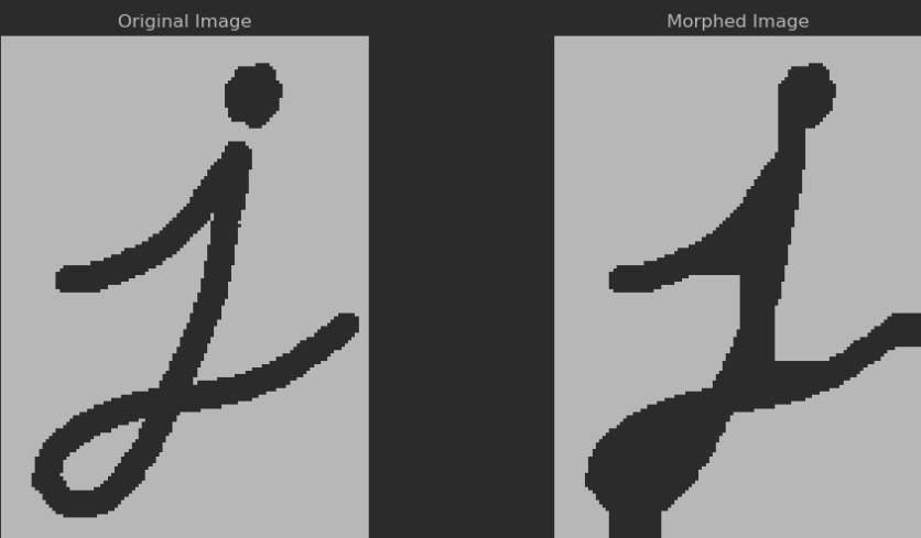
As you can see, the algorithm may be a bit too eager, as it merges parts of the letter with the image borders. However, for the crack bounding box detection problem, it will get the job done.
Returning to the find_boxes function, there’s a line that needs a bit of explanation: num_labels, labels, stats, centroids = cv2.connectedComponentsWithStats(binary_image, connectivity=8). The cv2 function called here is essentially a more complex version of the flood fill algorithm many of us learned in university. For those unfamiliar, here’s a quick explanation: flood fill iterates over a pixel matrix, pixel by pixel. When it encounters a pixel of interest (a white one), it expands in 4 or 8 directions and continues this process (in this case, the connectivity=8 argument allows it to expand in 8 directions). This way, the entire matrix is covered, and each connected cluster of pixels is identified.
The connectedComponentsWithStats function returns four things:
num_labels- how many separate objects have been detected?labels- segmentation mask matrix where different objects have different label number assignedstats- bounding boxes arraycentroids- center points of the bounding boxes
The labels are used a few lines later to identify the segmentation masks, which are then saved under the segmentation property of the COCO object. The stats are used to populate the bbox property, while the other two return values are disregarded. Near the end of the function, merge_adjacent_bboxes is called to ensure that any adjacent bounding boxes are merged together.
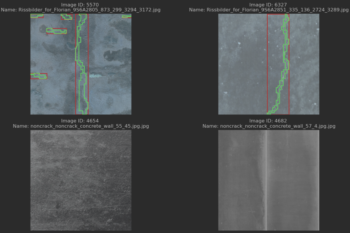
Testing
It’s always good to verify what our code produces, so I created another notebook for this purpose. It loads the COCO file and iterates over the annotations property, separating the annotations into two categories: those with bounding boxes and those without. It then randomly samples from both groups and displays the images, overlaying the detected segmentation masks and bounding boxes on top of them.
import json
import random
import os
import cv2
import numpy as np
import matplotlib.pyplot as plt

with open(os.path.join("data", "train", "coco_annotations.json"), "r") as f:
    coco_data = json.load(f)

annotations_with_bbox = [anno for anno in coco_data["annotations"] if anno["area"]]
annotations_without_bbox = [anno for anno in coco_data["annotations"] if not anno["area"]]
selected_with_bbox = random.sample(annotations_with_bbox, 8)
selected_without_bbox = random.sample(annotations_without_bbox, 4)
selected_annotations = selected_with_bbox + selected_without_bbox

images_dir = os.path.join("data", "train", "images")
rows, cols = 6, 2
subplot_width, subplot_height = 400, 400
figure_width = subplot_width * cols * 2 / 100
figure_height = subplot_height * rows / 100

plt.figure(figsize=(figure_width, figure_height))

for idx, annotation in enumerate(selected_annotations):
    plt.subplot(rows, cols, idx + 1)

    image_id = annotation["image_id"]
    image_info = next(img for img in coco_data["images"] if img["id"] == image_id)
    image_path = os.path.join(images_dir, image_info["file_name"])
    image = cv2.imread(image_path)
    image_rgb = cv2.cvtColor(image, cv2.COLOR_BGR2RGB)

    plt.imshow(image_rgb)

    image_annotations = [anno for anno in coco_data["annotations"] if anno["image_id"] == image_id]

    for anno in image_annotations:
        if anno["bbox"]:
            x, y, w, h = anno["bbox"]
            plt.gca().add_patch(plt.Rectangle((x, y), w, h, edgecolor='r', facecolor='none', linewidth=2))

        if anno["segmentation"]:
            for seg in anno["segmentation"]:
                seg_np = np.array(seg).reshape((-1, 2))
                plt.gca().add_patch(plt.Polygon(seg_np, edgecolor='g', facecolor='none', linewidth=2))

    plt.title(f"Image ID: {image_id} \nName: {image_info['file_name']}")
    plt.axis("off")

plt.tight_layout()
plt.show()
The effect is visible below:
Summary and next steps
It seems that the data engineering code I created in the first step does the job. It can correct some of the errors found in the dataset, effectively limiting the bounding box count, which should make training the neural networks easier. Next up is an implementation of the R-CNN architecture, as described in the paper.