Semantic search engines comparison, Part 2 - performance considerations
The last post got quite long, so I decided that splitting the rest of the series into smaller parts will be both: more readable and easier for me to do. So here it is, a very short post about ChromaDB. I will mention couple of facts from their official documentation for my future reference + make some experiments just for fun.
ChromaDB - Excerpts from the docs
You may remember what I said about ChromaDB - it’s a simple tech in its current state. It’s been designed for a single task, that is the vector search, and it does that task very well.
In the previous post you might have noticed the hnsw term used in the create_collection method call. hnsw (Hierarchical Navigable Small World Graphs) is an algorithm that ChromaDB (and Elasticsearch, not yet sure what PostgreSQL does, but I bet it’s the same) uses to search over embedding vectors. In their doc they give a link to a lib they incorporated into their product; that lib implements the hnsw algorithm. I could try explaining it, but when I googled it, I got the best search result, something way better than I could write, so here it is. TLDR; it’s O(log N). Pretty cool, huh?
ChromaDB’s documentation states that the index data must be kept in RAM. Additionally, it performs processing using the CPU, not the GPU, which came as a surprise to me. I haven’t delved deeply into the details, but my guess is that there’s nothing inherent in hnsw preventing it from running on a GPU. However, GPUs generally have less memory compared to RAM, and since we’re dealing with a database, space consumption is a significant factor. I hypothesize that moving data in batches between RAM and GPU memory, along with coordinating the search, would likely reduce the algorithm’s performance compared to running it directly on the CPU with RAM.
More than that, ChromaDB is single-threaded! That doesn’t have to be a very bad thing though, as Redis example teaches us (it’s also single threaded, but performant enough to be used as caching technology). It’s mentioned in the docs directly:
Although aspects of HNSW’s algorithm are multithreaded internally, only one thread can read or write to a given index at a time. For the most part, single-node Chroma is fundamentally single threaded. If a operation is executed while another is still in progress, it blocks until the first one is complete.
Elasticsearch - Excerpts from the docs
As a more mature technology, Elasticsearch offers some interesting features that the other engines lack. I’m talking about quantization. This process converts high-precision floating-point numbers (e.g., 32-bit floats) in the vector into lower-precision ones (e.g., 8 or 4-bit integers). This reduces the amount of RAM memory required to store the vectors and can accelerate similarity calculations because lower-precision operations are computationally cheaper. However, keep in mind that using lower-precision vectors will cause the searches to be less accurate but maybe that’s not something to be very worried about - at least for the int8 quantization (which is the default) the accuracy drop is negligible. The docs also mention that they can adapt to the data drift in order to keep the precision as high as it can be. This article contains a ton of useful information.
Sadly, ES is somewhat limited by one constraint. At the time of this writing the dims index parameter max value is 4096, which means you cannot store vectors longer than that in ES. That’s a pity because the newer GPT models produce 12k+ dimensional embeddings. It’s not an issue with ChromaDB though - that engine is only constrained by the integer size.
Similarly to ChromaDB, ES hnsw index needs to reside in memory in full. Or does it? Well, actually it doesn’t have to as described on this page, but if you keep some of your data on disk, performnace will be severely impacted. Still, if you have a big dataset that won’t fit into RAM, maybe that’s an ok option.
Apart from that ES is a nosql database that implements the idea of sharding that’s described like this in an AWS doc that I found:
Database sharding is the process of storing a large database across multiple machines. A single machine, or database server, can store and process only a limited amount of data. Database sharding overcomes this limitation by splitting data into smaller chunks, called shards, and storing them across several database servers. All database servers usually have the same underlying technologies, and they work together to store and process large volumes of data.
What it means is that you have the built-in capability of scaling out with a db such as ES. As for the similarity search - ES will perform an independent similarity search on each shard and then aggregate the results. This will incur some performance cost (aggregation + network traffic within the cluster). One thing to remember here is to keep track of the data distribution. If the data is spread unevenly, then some shards will be busier than others.
PostgreSQL - Excerpts from the docs
Postgres is yet another mature technology in this comparison serie. I need to admit - I’m a PostgreSQL fanboy. Honestly, after years of working with some alternative tech like Elasticsearch, MongoDB, Cassandra, Azure Cosmos DB and DynamoDB I really enjoy going back to what I learned over 20 years ago - just plain goddamn SQL - sometimes you just don’t need anything else :)
Starting where I left off in the ES section: sharding. If you ventured into the nosql world for several years and came back to PGSQL recently you may be surprised that it can be sharded now, using this extension for example. I haven’t really tried that, but it’s good to know that there’s now such an option available to the developers. And apart from that, database replication is also something you could use with PGSQL.
As for the performance tuning: you can’t really do much magic with the hnsw index other than quantizing the vectors like ES does, or lowering float precision of the numbers in them - that strategy is something that the pgvector extension employs. Both will lower the disk space footprint. As for the search speed - I’ll see if they do anything to it in this post.
As for something that will have a direct impact on the search speed, pgvector hnsw index implementation exposes the ef_search property. The docs are saying that its default value is 40 and changing it will affect the performance.
Side note: there’s also the IVFFlat index that the pgvector extension exposes, but since the other two engines only use hnsw describing it in a post such as this one wouldn’t make sense.
Indexing remarks
You probably noticed I’m not talking about the indexing process at all. In this series I didn’t really want to go into that because (at least in the apps I worked with) usually only a single big data seed/load is done at the project’s inception and when documents are added, there’s not that many of them. I thought that looking at the performance only from the search perspective would be much more useful for me in the future, but obviously if you’re reading this post trying to decide which engine to choose for your project and you expect that a lot of indexing will happen, you should also learn how fast this process is.
The code
Code here will contain some repeated lines (as compared to the previous post). I do that to give those repeated excerpts a bit more context and to refer directly to what I’m explaining. Let’s start with the docker definitions:
name: vectordbsservices

services:
  postgres:
    image: pgvector/pgvector:0.8.0-pg16
    environment:
      - POSTGRES_USER=vectors
      - POSTGRES_PASSWORD=vectors
      - POSTGRES_DB=vectors
      - POSTGRES_HOST_AUTH_METHOD=trust
      - PG_SHARED_BUFFERS=12GB
      - PG_EFFECTIVE_CACHE_SIZE=12GB
    ports:
      - "5435:5432"
    volumes:
      - vec_postgres_data:/var/lib/postgresql/data
      - ./scripts:/docker-entrypoint-initdb.d

  chromadb:
    image: chromadb/chroma:0.5.20
    volumes:
      - ./chromadb:/chroma/chroma
    environment:
      - IS_PERSISTENT=TRUE
      - PERSIST_DIRECTORY=/chroma/chroma
      - ANONYMIZED_TELEMETRY=${ANONYMIZED_TELEMETRY:-TRUE}
    ports:
      - "8123:8000"
    deploy:
      resources:
        limits:
          memory: 12g
        reservations:
          memory: 8g

  elasticsearch:
    image: docker.elastic.co/elasticsearch/elasticsearch:8.17.0
    environment:
      - discovery.type=single-node
      - ES_JAVA_OPTS=-Xms12g -Xmx12g
      - ELASTIC_PASSWORD=vectors
      - xpack.security.enabled=true
    ports:
      - "9200:9200"
      - "9300:9300"
    volumes:
      - esdata:/usr/share/elasticsearch/data
    restart: always

volumes:
  vec_postgres_data:
  esdata:
    driver: local
I’m making 12g of memory available for each engine. For Postgres there are more options, but they would mostly improve indexing; I didn’t use them because I wanted to avoid cluttering the docker-compose file. 12gb is well above what the datasets I’m using would require.
As for the python code, the interface notebook also contains code to measure the performance of each db:
engines = search_engine_box.options
models = model_box.options
queries = [
    "drunk football hooligans",
    "manifold hypothesis",
    "fuel prices growing",
    "climate change",
    "south america football news"
]
results = []

for engine in engines:
    suffixes = []

    if engine == "postgres":
        suffixes.extend([
            "-with-halfvec",
            "-ef-search-halved",
            "-with-halfvec-ef-search-halved"
        ])
    elif engine == "elasticsearch":
        suffixes.extend([
            "-with-quantization",
        ])

    for model, suffix, query in itertools.product(models, suffixes, queries):
        for i in range(30):
            try:
                _, elapsed_time = run_request(engine, model, query, suffix)

                results.append({
                    "engine": engine,
                    "model": f"{model}{suffix}",
                    "query": query,
                    "elapsed_time": elapsed_time
                })
            except Exception as e:
                print(f"Request failed for ({engine}, {model}, {suffix}, {query}): {e}")

df = pd.DataFrame(results)
summary_df = (df
              .groupby(["engine", "model"])
              .agg(
                  mean_time=("elapsed_time", "mean"),
                  std_time=("elapsed_time", "std"))
              .sort_values(by="mean_time", ascending=False)
              .reset_index())

summary_df
This code defines five queries which are then run thirty times for each model+engine combination to obtain a statically significant result. Then the results are aggregated and two numbers are extracted that will inform us of the experiment results. In order to make this a fair competition I had to change ChromaDB and Elasticsearch related code slightly - both of those places were pulling data from pg database because of a mistake I made (saving normalized data to those databases instead of sacing the original data). The “fix” was to comment out that code. Results below:
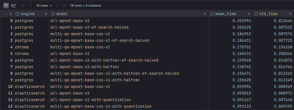
Summary
It looks like Elasticsearch beats the other two engines by a big margin even without any quantization applied. This comes as a surprise to me because I thought that ChromaDB would shine in this comparison since it’s a new product with no legacy code in it (ES has to have it, it’s just too mature not to).