Detecting Conformance to Benford’s Law Using Apache Spark
Before diving back into neural network topics, I figured I needed a bit of space to breathe - away from AI, transformers, and multiple-hour-long wait times. For that, I picked a simple idea: checking if a number series aligns with a certain statistical distribution. On its own, that would be a pretty basic task, so I decided to complicate it in two ways: by using Apache Spark and by going with a distribution that’s not as widely known as, say, the normal distribution. Enter Benford’s distribution - and Benford’s law it’s built upon.
Why Apache Spark and not Pandas? The reason is simple - laziness. I already had most of the code ready from one of my older passion projects. The only thing I had to change was swapping in Benford’s distribution instead of the one I used back then.
Side note: from what I’ve seen on the internet, this is often used for fraud detection in banking, though it’s by no means limited to that domain. In this post, I’ll use some synthetic data to demonstrate the calculations.
WTH is Benford’s Law?!
First, some theory. Benford’s Law states that if you take the first digit from each number in a series, the digits should appear with certain precalculated probabilities. For example, the digit 1 should appear about 30% of the time, digit 2 about 17.5%, all the way up to digit 9, which according to Benford’s Law should appear only around 4.5% of the time. This corresponds to the Benford distribution known in statistics. It’s represented by this formula:
\[\begin{aligned} P(d) = \log_{10}\left(1 + \frac{1}{d}\right), \quad d = 1, 2, \dots, 9 \end{aligned}\]And looks like this:
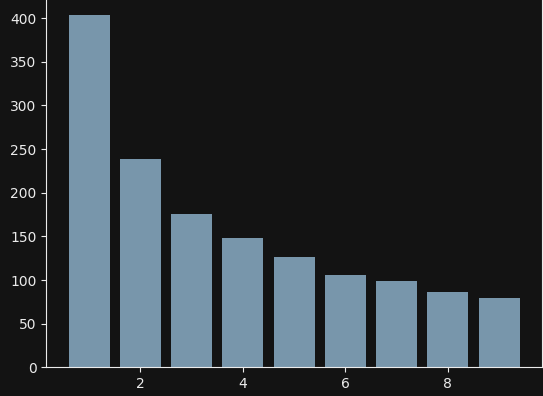
It shows a plot generated off of values produced by this function:
def generate_benford_values(n_days: int = 365 * 4) -> list[int]:
    multiplier = np.log(100)

    return list(
        np.exp(multiplier * np.random.rand(n_days)).astype(int)
    )
It actually produces a log-uniform distribution, but the leading digits conform to Benford’s Law, that’s why I used it.
Side note: obviously not all natural phenomena will produce number series conforming to this law, but some will (like cash flows being inspected in fraud detection algorithms).
Testing
In data analysis looking at the data is the first step. In this case I didn’t have any data, so I generated some for the experiment using these functions:
def generate_uniform_values(n_data_points: int = 365 * 4) -> list[int]:
    values = []
    magnitudes = [4, 5, 6, 7]  # 10^4 to 10^7 range

    for _ in range(n_data_points):
        # Pick a random first digit with uniform probability
        first_digit = random.randint(1, 9)
        # Pick a random magnitude
        magnitude = random.choice(magnitudes)
        # Generate a number starting with that digit
        # For digit d and magnitude m: range is [d * 10^(m-1), (d+1) * 10^(m-1) - 1]
        min_val = first_digit * (10 ** (magnitude - 1))
        max_val = (first_digit + 1) * (10 ** (magnitude - 1)) - 1
        value = random.randint(min_val, max_val)

        values.append(value)

    return value
Why the 365 * 4 multiplication? In this experiment, I wanted a year’s worth of data where each day produces 4 data points. As for the loop, it iterates over the given range, picks a random number between 1 and 9, chooses a magnitude (whether it’s 10,000 or 10,000,000 doesn’t really matter - everything could’ve just been within a fixed range like [1, 1000]), selects limits that should constrain the randomly chosen number, and appends it to a list.
Then, to visualize what’s been produced I use this code:
def get_first_digits(values: list[int]) -> tuple[list[int], list[int], list[int]]:
    first_digits = list(map(lambda x: int(str(x)[0]), values))
    digit_occurences = dict(Counter(first_digits))
    keys = list(digit_occurences.keys())
    values = list(digit_occurences.values())

    return first_digits, keys, values


u_values = generate_uniform_values()
u_first_digits, u_keys, u_values = get_first_digits(u_values)

plt.bar(u_keys, u_values)
I also created three more functions to generate variable set of test cases that I will later use:
import numpy as np
import random

def generate_biased_values(n_days: int = 365 * 4) -> list[int]:
    scales = [1e4, 1e5, 1e6, 1e7]
    values = []

    for _ in range(n_days):
        scale = random.choice(scales)

        if random.random() < 0.7:  # natural distribution
            value = int(np.random.lognormal(mean=np.log(scale), sigma=1.5))
        else:  # biased branch
            magnitude = int(np.log10(scale))
            r = random.random()

            if r < 0.4:  # overrepresent digit 5
                value = random.randint(5_000_000, 5_999_999)
            elif r < 0.7:  # underrepresent digit 1 favoring 2, 3, 4
                digit = random.choice([2, 3, 4])
                value = random.randint(digit * 10 ** magnitude,
                                       (digit + 1) * 10 ** magnitude - 1)
            else:  # overrepresent digit 9
                value = random.randint(9 * 10 ** (magnitude - 1),
                                       10 ** magnitude - 1)

        value = max(10_000, min(100_000_000, value))

        values.append(value)

    return values


def generate_lognormal_values(n_days: int = 365 * 4) -> list[int]:
    return list(
        np.random.lognormal(mean=np.log(5000), sigma=0.25, size=n_days).astype(int)
    )


def generate_benford_values(n_days: int = 365 * 4) -> list[int]:
    multiplier = np.log(100)

    return list(
        np.exp(multiplier * np.random.rand(n_days)).astype(int)
    )
generate_benford_values has been described earlier, so I’ll skip it here. As for the lognormal value generator - I chose lognormal because it generates strictly positive values. I could have just used a normal distribution, but it can produce negatives, even with a very large loc parameter. Since we’ll be considering str(x)[0] in the first digit selection function, it’s more intuitive to use something strictly positive from the start.
generate_biased_values produces values from a lognormal distribution 70% of the time, and 30% of the time it overrepresents certain numbers. The magnitude calculations are there only to make the overall number range more spread out, but it could just as well be simplified to use a fixed range (like in the generate_uniform_values function).
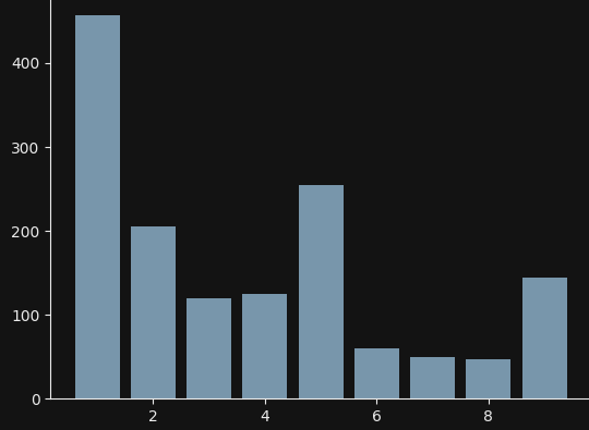
This is how the biased distribution can look like:
I also defined a function to check what does the scipy.stats.chisquare function think about them:
def get_chisquare(first_digits: list[int]) -> tuple[float, float]:
    benford_probs = get_benford_probabilities()
    observed_counts = np.zeros(9)

    for digit in first_digits:
        observed_counts[digit - 1] += 1

    expected_counts = benford_probs * len(first_digits)
    chi_stat, p_value = chisquare(
        f_obs=observed_counts,
        f_exp=expected_counts
    )

    return chi_stat, p_value
After feeding it first digits for each distribution I got these results:
- Uniform: (np.float64(701.2662324951431), np.float64(3.820331560700687e-146))
- Biased: (np.float64(329.04613868697993), np.float64(2.673073644629964e-66))
- Lognormal: (np.float64(2250.8987402440307), np.float64(0.0))
- Benford: (np.float64(10.862339416528645), np.float64(0.2096219090178658))
The chisquare test produced very high chi_stat and very low p_value’s for the first three ones which means that there’s almost zero probability for them to come from benford distribution, contrary to the last one.
Since this whole idea came from one of my old apps, I also wanted to show a unit test I wrote, that utilizes the code show earlier. There will be some references to components that I haven’t defined yet - I’ll do that shortly:
class MockSharedSparkSession(SharedSparkSession):
    def get(self, **kwargs) -> SparkSession:
        return (
            SparkSession
            .builder
            .master("local[*]")
            .appName("unit-test")
            .config("spark.sql.shuffle.partitions", "1")
            .config("spark.sql.adaptive.enabled", "false")
            .getOrCreate()
        )


spark_session = MockSharedSparkSession()


@pytest.fixture
def sut():
    return BenfordAnalysis(spark_session)


def create_data_frame(volumes: list[int]) -> DataFrame:
    start_date = datetime.now(timezone.utc) - timedelta(days=365)
    data = []
    current_date = start_date

    for day in range(len(volumes) // 4):
        date_only = current_date.date()
        times = [
            current_date.replace(hour=10),
            current_date.replace(hour=12),
            current_date.replace(hour=14),
            current_date.replace(hour=16),
        ]
        day_values = values[day * 4:(day + 1) * 4]

        for ts_dt, value in zip(times, day_values):
            ts = int(ts_dt.timestamp() * 1000)
            data.append((
                date_only,
                ts,
                ts_dt,
                Decimal(str(value))
            ))

        current_date += timedelta(days=1)

    schema = StructType([
        StructField("date", DateType(), False),
        StructField("ts", LongType(), False),
        StructField("datetime_", TimestampType(), False),
        StructField("volume", DecimalType(20, 0), True),
    ])

    return spark_session.get().createDataFrame(data, schema)


@pytest.mark.parametrize(
    "data_frame,expected_label",
    [
        (create_data_frame(generate_uniform_values()), "high"),
        (create_data_frame(generate_biased_values()), "high"),
        (create_data_frame(generate_lognormal_values()), "high"),
        (create_data_frame(generate_benford_values()), "low"),
    ]
)
def test_benford_analysis_command_threshold(
        sut: BenfordAnalysis,
        data_frame: DataFrame,
        expected_label: str,
        monkeypatch
):
    monkeypatch.setattr(sut, "_get_initial_df", lambda t: data_frame)

    result = sut.run()
    chi_series = result[0]["chi_sq_series"]
    chi_stat = float(chi_series[0])

    if expected_label == "high":
        assert chi_stat > 15, f"Chi-square {chi_stat} unexpectedly low"
    else:
        assert chi_stat < 15, f"Chi-square {chi_stat} unexpectedly high"
A rather simple unit test - it generates three distributions that are different from Benford’s and one that actually is the Benford distribution. In the beginning I was tempted to compare the chi_stat to some actual numbers (using margins), since it will be of different value for each of the parameters, but given the partially random nature of the generate_*_values functions, it would be very hard to find a good range that wouldn’t cause the test to fail from time to time.
The code
The code is rather involved - it’s a bunch of pyspark queries, so I’ll describe the BenfordAnalysis class method by method.
def run(self) -> dict[str, str | int | float]:
    initial_df = self._get_initial_df()

    logger.info(f"Intraday count is: {initial_df.count()}")

    analysis_df = self._get_analysis_df(initial_df)

    logger.info(f"Analysis count is: {analysis_df.count()}")

    problematic_results = BenfordAnalysisCommand._get_problematic_results(analysis_df)

    logger.info(f"CHI-squared count is: {problematic_results.count()}")

    result = problematic_results.toPandas().to_dict(orient="records")

    return result[0]
This is the entry point of my logic. First, it gets the initial dataframe - while doing that, one of the dataframes passed in as parameters to the test is used. Then it runs the analysis method, which extracts the first digits (among other things), and after that another method takes care of the chi-square calculation. I’m not showing the _get_initial_df method because it simply selects the data.
Side note: before I describe the next method, an important remark: this code assumes there’s data only for a single entity - be it a bank account, medical study, or something else. However, it would work if there were multiple such entities in which case the grouping would have to be done by some unique identifier of that entity.
Creating the initial dataframe
A word of introduction: a lot of this code is just a quirk of my implementation. Splitting the data into quarters, then downweighting p-values based on their recency - obviously you could do just fine without them, it’s just what I needed in my app. I also decided to not simplify those parts because they don’t add a lot of mental overhead, while at the same time they just seem interesting (to me ;) ). Back to the code:
def _get_analysis_df(self, df: DataFrame) -> DataFrame:
    logger.info("Running Benford analysis...")

    MIN_QUARTERS = 4
    now = datetime.datetime.now(datetime.UTC)
    df = (
        df
        .withColumn(_Columns.CURRENT_YEAR, F.year(_Columns.DATETIME_))
        .withColumn(_Columns.CURRENT_QUARTER, F.quarter(_Columns.DATETIME_))
        .withColumn(_Columns.END_YEAR, F.year(F.lit(now)))
        .withColumn(_Columns.END_QUARTER, F.quarter(F.lit(now)))
        .withColumn(
            _Columns.QUARTERS_FROM_END,
            (F.col(_Columns.END_YEAR) - F.col(_Columns.CURRENT_YEAR)) * 4 +
            (F.col(_Columns.END_QUARTER) - F.col(_Columns.CURRENT_QUARTER))
        )
        .withColumn(_Columns.FIRST_DIGIT,
                    F.expr(r"regexp_extract(cast(abs(volume) as string), '([^0.])', 1)"))
    )
    num_quarters = (
        df
        .select(F.countDistinct(_Columns.QUARTERS_FROM_END).alias("cnt"))
        .first()["cnt"]
    )

    if num_quarters < MIN_QUARTERS:
        logger.warning(f"Data has fewer than {MIN_QUARTERS} quarters, returning empty DataFrame")

        return self._spark.createDataFrame([], schema=[
            _Columns.QUARTERS_FROM_END, _Columns.DIGIT, _Columns.COUNT, _Columns.TOTAL,
            _Columns.EXPECTED, _Columns.EXPECTED_COUNT, _Columns.CHI_SQ_TERM
        ])

    benford_probs = {str(d): np.log10(1 + 1 / d) for d in range(1, 10)}
    benford_df = self._spark.createDataFrame(
        [(k, float(v)) for k, v in benford_probs.items()],
        [_Columns.DIGIT, _Columns.EXPECTED]
    )
    pivoted_counts = (
        df
        .groupBy(_Columns.QUARTERS_FROM_END)
        .pivot(_Columns.FIRST_DIGIT, [str(i) for i in range(1, 10)])
        .count()
        .na.fill(0)
    )
    full_digit_counts = pivoted_counts.select(
        _Columns.QUARTERS_FROM_END,
        F.expr(
            f"stack(9, '1', `1`, '2', `2`, '3', `3`, '4', `4`, '5', `5`, '6', `6`, '7', `7`, '8', `8`, '9', `9`) as ({_Columns.DIGIT}, {_Columns.COUNT})")
    ).cache()
    total_counts = full_digit_counts.groupBy(_Columns.QUARTERS_FROM_END).agg(
        F.sum(_Columns.COUNT).alias(_Columns.TOTAL)
    )
    analysis_df = (
        full_digit_counts
        .join(total_counts, [_Columns.QUARTERS_FROM_END])
        .join(benford_df, _Columns.DIGIT)
        .withColumn(_Columns.EXPECTED_COUNT, F.col(_Columns.EXPECTED) * F.col(_Columns.TOTAL))
        .withColumn(_Columns.CHI_SQ_TERM,
                    (F.col(_Columns.COUNT) - F.col(_Columns.EXPECTED_COUNT)) ** 2 / F.col(_Columns.EXPECTED_COUNT))
    )

    full_digit_counts.unpersist()

    return analysis_df
Now this is where things start to get interesting. Btw. that’s the full method in case you’d like to understand it without my explanations.
Anysways, the second line sets a constant MIN_QUARTERS. In the beginning of this post I mentioned this all comes from one of my passion projects. In that project I assumed I will check the data while bucketing it into calendar quarters, to also see if there’s a seasonality in the numbers. And so, the first df = ( expression does just that - it calculates where in the “quarter” space is the given datapoint with this part:
(F.col(_Columns.END_YEAR) - F.col(_Columns.CURRENT_YEAR)) * 4 +
(F.col(_Columns.END_QUARTER) - F.col(_Columns.CURRENT_QUARTER))
It first considers the year of the datapoint - if it’s the current one, it will be 0 * 4 = 0 - and then adds the number of quarters from the one we’re currently in. So if it’s August, we’re in the third quarter of the year, and if the datapoint comes from January, that calculation will give us 3 - 1 = 2, meaning the considered quarter is two quarters away from the current one. What this does is assign a unique “quarters from end” label. For example, if it’s December 2025, data from this month will fall into bucket #0, and data from December 2024 will fall into bucket #4.
.withColumn(_Columns.FIRST_DIGIT,
            F.expr(r"regexp_extract(cast(abs(volume) as string), '([^0.])', 1)"))
I guess this is rather self-explanatory - it just pulls the first digit from the number for later analysis (and it’s actually the core expression in this whole code :D). The next part checks if there’s enough data to perform the analysis and returns an empty dataframe in case there’s not. Moving on to the part after that:
benford_probs = {str(d): np.log10(1 + 1 / d) for d in range(1, 10)}
benford_df = self._spark.createDataFrame(
    [(k, float(v)) for k, v in benford_probs.items()],
    [_Columns.DIGIT, _Columns.EXPECTED]
)
This code creates the distribution described in the “WTH is Benford’s Law?!” section and creates a dataframe holding it.
The fragment that follows does the following:
- It groups the data by the quarter info and creates a pivot table where columns are the first digits - in case some digit is missing, it will be present because of that second method argument. So after pivoting, the data could look like this:
quarters_from_end | 1  | 2    | 3  | 4    | 5    | 6    | 7    | 8 | 9
1                 | 50 | 30   | 20 | null | null | null | null | 8 | null
2                 | 45 | null | 25 | null | null | null | null | 0 | 6
And after the .na.fill(0) call it could look like this:
quarters_from_end | 1  | 2 | 3  | 4 | 5 | 6 | 7 | 8 | 9
1                 | 50 | 30| 20 | 0 | 0 | 0 | 0 | 8 | 0
2                 | 45 | 0 | 25 | 0 | 0 | 0 | 0 | 0 | 6
- The next call unpivots the data. The
stackSpark function call looks weird, but its interface is this:
stack(n, 'label1', take_value_from_col_no1, 'label2', take_value_from_col_no2, ..., 'labeln', take_value_from_col_no_n)
So the exact expression that I used says:
- Create 9 rows from each input row
- Row 1: digit=’1’, count=value from column 1
- Row 2: digit=’2’, count=value from column 2
- Row 3: digit=’3’, count=value from column 3
- …and so on
There is at least a few other ways of achieving the same goal. E.g. I could have used a cross join between quarters and first digits, and join that dataframe with another one that would group by quarters from end and first digit, and finally fill the missing rows with 0’s, but that’s just more work, so… Pivot tables FTW!
total_countsdf just sums all the datapoints within each quarter.analysis_dfjoinstotal_countsandbenford_df, and calculates the absolute number of occurrences we should expect for each digit in each quarter. Then it uses that in the chi square formula to obtain the final result.
Calculating the remaining chi square elements
No statystical analysis would be complete without calculating p-values and this one is no different. For that I created this udf to be used in a method I’ll show next:
@udf(returnType=DoubleType())
def chi2_pvalue(chi_sq_stat):
    return float(1 - chi2.cdf(chi_sq_stat, df=8))
It uses the scipy’s chi2 function to obtain p-value from the previously calculated chi-square statistic. It’s then used as the input to another udf:
@udf(returnType=FloatType())
def compute_weighted_deviation_confidence(p_values):
    if len(p_values) == 0:
        return 0.0

    total_weight = 0.0
    deviation_weight = 0.0

    for i, p_value in enumerate(p_values):
        weight = 0.8 ** i
        total_weight += weight

        if p_value < 0.05:
            deviation_weight += weight

    return deviation_weight / total_weight if total_weight > 0 else 0.0
What it does, is it looks at the p-values and downweights them based on recency and returns a confidence score which is just the averaged deviation sum. These two udfs are used in a method that wraps-up the whole logic of benford analysis:
def _get_problematic_results(analysis_df: DataFrame) -> DataFrame:
    chi_sq_results = (
        analysis_df
        .groupBy(_Columns.QUARTERS_FROM_END)
        .agg(F.sum(_Columns.CHI_SQ_TERM).alias(_Columns.CHI_SQ_STATISTIC))
        .withColumn("p_value", chi2_pvalue(_Columns.CHI_SQ_STATISTIC))
        .withColumn("significant_05", F.col("p_value") < 0.05)
    )
    ordered = chi_sq_results.orderBy(F.col(_Columns.QUARTERS_FROM_END).desc())
    chi_sq_series = (
        ordered
        .agg(
            F.collect_list(_Columns.CHI_SQ_STATISTIC).alias(_Columns.CHI_SQ_SERIES),
            F.collect_list("p_value").alias("p_value_series")
        )
    )
    deviation_scores = (
        chi_sq_series
        .withColumn(_Columns.DEVIATION_CONFIDENCE,
                    compute_weighted_deviation_confidence("p_value_series", _Columns.CHI_SQ_SERIES))
        .withColumn("n_quarters", F.size(_Columns.CHI_SQ_SERIES))
    )
    likely_problematic = deviation_scores.filter(
        F.col(_Columns.DEVIATION_CONFIDENCE) >= F.lit(0.5))
    )

    return likely_problematic
This time all the magic was residing in the udf and this function simply returns a dataframe that is filtered by the confidence score. If the p-value was small enough, then the null hypothesis was rejected for that quarter (null hypothesis being: the data follows Benford’s Law for that quarter). Btw. that filter call is yet another quirk of my code. In other case it could be useful to actually show all the results.
Summary
I’m tempted to write a similar post about doing the same in Pandas, just as a practice. It took me some time to understand my old code anew and in the end I was missing AI topics, so the next post will probably come back to that subject. I hope you enjoyed!