Denoising autoencoders, Part 3 - improving the denoising quality with a custom loss function
In the previous post, I said I probably wouldn’t come back to this topic soon, but I couldn’t stop thinking that this series wouldn’t be complete until I investigated how my final architecture “thinks” and, depending on what I saw, whether there might still be some low-hanging fruit to harvest in this project. Also, when I zoomed in on the denoised images, it became clear than they are blurry - so of them REALLY blurry. Could something be done with that? …And so I arrived at the idea of using the pytorch-grad-cam library to see what activates my network, which in turn guided my next steps.
So… WHAT IS THAT?!
Glad you asked! From what I read on the internet, explainability has been one of the hottest topics in AI for several years now. We - the neural networks architects - love how our code turns impossible problems into solutions, but explaining why a certain architecture made certain decision has been a problem since the dawn of time. Obviously looking at how single neurons work is not really productive, as the “thinking” of neural network happens when they cooperate. That means they need to be analyzed on a higher level. That’s why some explainability frameworks have been introduced. One of them is the one I mentioned in the introduction - pytorch-grad-cam. The idea is simple - give it a trained model instance, layers that you want to inspect and sample images. It will give back a heat map representing the image fragments that activated the inspected layers the most.
There’s one caveat - the library wants its user to give it some targets. That’s easy when the task at hand is about classification, object detection, or semantic segmentation, because the targets are available. In the case of a denoising task, there’s no such natural target because the network’s goal is not to find something on an image but rather make the image better-looking. That’s why an artificial target needs to be passed in (gradients have to be calculated with respect to something). The result of that is that there’s some manual work to be done around using various “cameras” exposed by this lib.
The code - inspecting the activations
As the winner architecture from the last post consisted of two subnetworks, I was interested in learning what does the ViT network thinks is important and then comparing that with the autoencoder module. So here comes the first of those manual steps - wrapping ViT in another module:
class ViTWrapper(nn.Module):
    def __init__(self, vit_model):
        super().__init__()

        self.vit = vit_model

    def forward(self, pixel_values):
        # outputs = self.vit(pixel_values=pixel_values)
        # patch_tokens = outputs.last_hidden_state[:, 1:, :]
        #
        # return torch.norm(patch_tokens, dim=2).mean(dim=1, keepdim=True)
        outputs = self.vit(pixel_values=pixel_values)
        patch_tokens = outputs.last_hidden_state[:, 1:, :]

        return patch_tokens.mean(dim=[1, 2], keepdim=True)
Why do I even do it? Well, that’s all because of that missing natural target. If there’s no object on the image that would be of interest to the training process and instead it’s the image as a whole that is the object of interest, I had to decide what general trait of an image I want to focus on to later show via the camera. In that code snippet you can see two alternatives that would result in very different visual outcomes. The commented-out one is the L2 norm. Using it would make strong features stand out. Strong features could be the cracks that are visible on my images. That was my expectation, but in reality big parts of the image were glowing red, which means it was not underlining anything in particular that would be of interest for the network. I switched to mean calculation and it made a world of difference (mean answers the question: “what contributes to the average activation?”).
Before I show the results, the rest of the code:
def run_cam(vit_input: torch.Tensor, targets: list[torch.nn.Module], cam: BaseCAM, name: str, do_filter: bool = False) -> None:
    cam_data = cam(input_tensor=vit_input, targets=targets)
    lower_threshold = 0.4
    upper_threshold = 0.9

    if do_filter:
        cam_data = cam_data[0]
        cam_data_filtered = np.where(
            (cam_data >= lower_threshold) & (cam_data <= upper_threshold),
            cam_data,
            0
        )

        if cam_data_filtered.max() > 0:
            non_zero_mask = cam_data_filtered > 0
            min_val = cam_data_filtered[non_zero_mask].min()
            max_val = cam_data_filtered[non_zero_mask].max()
            cam_data_final = np.zeros_like(cam_data_filtered)
            cam_data_final[non_zero_mask] = (cam_data_filtered[non_zero_mask] - min_val) / (max_val - min_val + 1e-8)
        else:
            cam_data_final = cam_data_filtered
    else:
        cam_data_final = cam_data[0]

    img_np = noisy_img.permute(1, 2, 0).numpy()
    img_np = (img_np - img_np.min()) / (img_np.max() - img_np.min() + 1e-8)

    overlay = show_cam_on_image(img_np.astype(np.float32), cam_data_final, use_rgb=True)

    plt.figure(figsize=(15, 5))
    plt.subplot(1, 3, 1)
    plt.imshow(img_np)
    plt.title("Input Noisy Image")
    plt.axis("off")
    plt.subplot(1, 3, 2)
    plt.imshow(cam_data_final, cmap='jet', vmin=0, vmax=1)
    plt.title(f"{name} Heatmap range")
    plt.colorbar()
    plt.axis("off")
    plt.subplot(1, 3, 3)
    plt.imshow(overlay)
    plt.title(f"{name} Overlay on ViT")
    plt.axis("off")
    plt.tight_layout()
    plt.show()
That if statement looks interesting, right? I mentioned this two times already - there’s no natural target here. No natural target -> the full image will be considered as the target by the cam. However, even in that case, some parts will stand out anyway, but given the small color difference, it’s not easy to see them. That’s why I decided to use some color thresholding - I noticed that objects in that range were not picked randomly.
with EigenCAM(model=wrapped_model, target_layers=target_layers, reshape_transform=vit_reshape_transform) as eigen_cam:
    with KPCA_CAM(model=wrapped_model, target_layers=target_layers, reshape_transform=vit_reshape_transform) as kpca_cam:

        for cnt in range(0, 10):
            vit_input = vit_noisy[cnt].unsqueeze(0).to(device)
            noisy_img = noisy[cnt].cpu()

            vit_input.requires_grad_()

            targets = [ClassifierOutputTarget(0)]

            run_cam(vit_input, targets, eigen_cam, name="Eigen")
            run_cam(vit_input, targets, kpca_cam, name="KPCA")
            print("=" * 100)
Why EigenCAM and KPCA_CAM? Actually, I used all of them and those two were showing something interesting. What’s even more interesting is that their results are - to a degree - complementary:
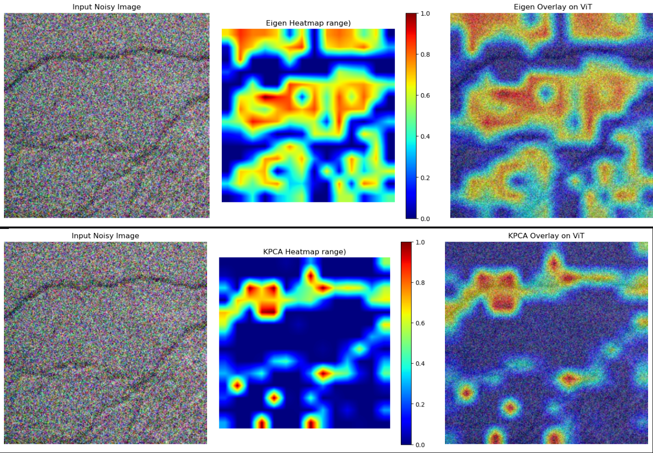
I gotta be honest - I cherry-picked this example, because most of the other images were rather random (but that’s expected!). But even with this cherry picking, it shows that ViT itself can “see” some bigger image traits, even though it was pretrained on a much different dataset. However, it gets more interesting when the autoencoder activations are visualized:

They are not as bright, and not complementary anymore. Also, it seems that the U-Net didn’t really pay attention to the cracks.
This is the moment when I finished my visual analysis and summed it up with: Okay, so ViT attends to the fragments that show cracks, and then the CNN module tones those features down. Is that good or bad? Well, the task was to denoise the images, not to denoise the cracks, and even though this is kind of weird, the overall process makes the result better (ViT + U-Net did a much better job than any other variation I tried). But what would happen if I pushed the network to focus on the features that activated ViT the most? That wouldn’t work. Some cracks are very small, so focusing on them could potentially make images better in the regions they occupy, but perhaps worse in the remaining ones. Hmm… But what if I focused on the edges? The images in my dataset are basically textures - asphalt, concrete, sand-like stuff, etc. There are visible edges between cracks and the other parts, but also between different elements of the images. For example, there are some stone-like pieces on top of sand; also, the asphalt material isn’t all black. Could focusing on that give some kind of visual quality boost?
The code - first attempts on sharpening the results
That’s how I arrived at the idea of a custom loss function that would penalize color differences between different colored regions. Cracks stand out from what they are on, stones look different from the material they are on, those small grains of whatever that asphalt surfaces have also differ from the rest of the texture.
But before I get to that, a word of explanation about the intuition I learned for MSE loss: In the introduction I mentioned the blurriness problem that occurs with MSE loss during training. MSE computes the mean squared difference between predictions and targets, but the optimization process creates a bias toward conservative predictions. When there’s uncertainty about the correct pixel value - such as when reconstructing details from noisy images - MSE’s squared penalty makes the network risk-averse. Instead of making bold predictions that might occasionally be very wrong, the network learns to predict ‘safe’ values that minimize the worst-case squared error. This leads to predictions that approximate the mean of possible target values. For example, if a pixel could be either 3 or 12 depending on the true underlying detail, MSE encourages the network to predict something closer to 7 or 8 - a compromise that keeps the squared error relatively low regardless of which value is actually correct. While this minimizes the loss function, it produces smooth, averaged-looking results. This optimization behavior, is what causes the blurriness and color desaturation we observe in MSE-trained denoising networks. Some of them, at least, or rather: trained by me ;)
Coming back to the code - I decided to create a variable that would hold windowed (with overlap) color-difference scores in the form of a dictionary. Why windowed? Well, color-difference scores on full images would be rather pointless - all useful information would be lost by using an average (in the end, the differences have to be flattened somehow). So color differences within a set of windows make much more sense.
Now, why the overlaps? To keep even more useful information. To visualize it: if you color one square in a notebook black and leave its neighbor white, and you pick the window size to be equal to the size of such a square, the average color difference within both squares would be zero. But if you slide the window by half the square size, you’ll get [0, INFORMATIVE_VALUE, 0]. That’s similar to how Conv2d layers work when you use different kernel-size and padding parameters. At least, that’s the intuition I used:
def calculate_sharpness_score(channel_slices: list[torch.Tensor]) -> float:
    total_scores = []

    for slice_tensor in channel_slices:
        # Horizontal differences (each pixel vs right neighbor)
        horizontal_diff = torch.abs(slice_tensor[:, :-1] - slice_tensor[:, 1:])
        # Vertical differences (each pixel vs bottom neighbor)
        vertical_diff = torch.abs(slice_tensor[:-1, :] - slice_tensor[1:, :])
        # Diagonal differences (top-left to bottom-right)
        diagonal1_diff = torch.abs(slice_tensor[:-1, :-1] - slice_tensor[1:, 1:])
        # Diagonal differences (top-right to bottom-left)
        diagonal2_diff = torch.abs(slice_tensor[:-1, 1:] - slice_tensor[1:, :-1])
        # Sum all differences for this channel
        channel_score = (horizontal_diff.sum() + vertical_diff.sum() + diagonal1_diff.sum() + diagonal2_diff.sum())

        total_scores.append(channel_score)

    average_score = torch.stack(total_scores).mean()

    return average_score.item()


def build_offline_cache(dataset: HybridDenoisingDataset, window_size: int) -> dict[str, list[float]]:
    cache = {}
    step_size = window_size // 2

    for noisy_image, clean_image, vit_noisy, filename in dataset:
        cache[filename] = []

        for x in range(0, clean_image.shape[1], step_size):
            for y in range(0, clean_image.shape[2], step_size):
                channel_slices = []

                for c in range(0, 3):
                    channel_array = clean_image[c]
                    slice = channel_array[x:x + window_size, y:y + window_size]

                    channel_slices.append(slice)

                sharpness_score = calculate_sharpness_score(channel_slices)

                cache[filename].append((x, y, sharpness_score))

    return cache
The function doing the actual calculations checks the neighbors horizontally, vertically and diagonally. It’s invoked by build_offline_cache over all channels. Obviously using such an explicit code would mean that the process of building the offline cache would take ages (8 minutes on my PC), so vectorized versions are more preferable:
def calculate_sharpness_score_vectorized(windows) -> torch.Tensor:
    horizontal_diff = torch.abs(windows[:, :, :, :, :-1] - windows[:, :, :, :, 1:])
    vertical_diff = torch.abs(windows[:, :, :, :-1, :] - windows[:, :, :, 1:, :])
    diagonal1_diff = torch.abs(windows[:, :, :, :-1, :-1] - windows[:, :, :, 1:, 1:])
    diagonal2_diff = torch.abs(windows[:, :, :, :-1, 1:] - windows[:, :, :, 1:, :-1])
    # Sum across spatial dimensions and average across channels
    total_diff = (horizontal_diff.sum(dim=(3,4)) + vertical_diff.sum(dim=(3,4)) +
                  diagonal1_diff.sum(dim=(3,4)) + diagonal2_diff.sum(dim=(3,4)))

    # Average across channels: (3, num_h_windows, num_w_windows) -> (num_h_windows, num_w_windows)
    return total_diff.mean(dim=0)


def build_offline_cache_optimized(dataset: HybridDenoisingDataset, window_size: int) -> dict[str, list[tuple[float, float, float]]]:
    cache = {}
    step_size = window_size // 2

    for noisy_image, clean_image, vit_noisy, filename in dataset:
        cache[filename] = []
        windows = clean_image.unfold(1, window_size, step_size).unfold(2, window_size, step_size)
        sharpness_scores = calculate_sharpness_score_vectorized(windows)
        num_h_windows, num_w_windows = windows.shape[1], windows.shape[2]

        for h_idx in range(num_h_windows):
            for w_idx in range(num_w_windows):
                x = h_idx * step_size
                y = w_idx * step_size
                score = sharpness_scores[h_idx, w_idx].item()

                cache[filename].append((x, y, score))

    return cache
Two for loops down, and the execution time went from 8 minutes to 43 seconds. Sweet. The loss function definition is as follows:
class RegionalSharpnessLoss(nn.Module):
    def __init__(self, cache: dict, window_size: int, step_size: int):
        super().__init__()

        self.cache = cache
        self.window_size = window_size
        self.step_size = step_size
        self.processed_cache = {}

        for filename, data in cache.items():
            scores = [score for x, y, score in data]
            scores = sorted(scores, reverse=True)
            self.processed_cache[filename] = torch.tensor(scores, device='cuda')

    def forward(self, outputs: torch.Tensor, _: torch.Tensor, filenames: list[str]) -> torch.Tensor:
        batch_losses = []

        for idx, filename in enumerate(filenames):
            output_score = calculate_sharpness_score_vectorized(
                outputs[idx]
                .unfold(1, self.window_size, self.step_size)
                .unfold(2, self.window_size, self.step_size)
            ).flatten()
            output_score = torch.sort(output_score, descending=True)[0]
            target_score = self.processed_cache[filename]

            batch_losses.append(torch.mean(torch.abs(output_score - target_score)))

        raw_loss = torch.stack(batch_losses).mean()
        normalized_loss = raw_loss / 1000.0

        return normalized_loss
It precalculates the processed_cache attribute to save some time after training (eg. it sorts using the sorted built-in, which means that this op is done on CPU - it would slow down training process significantly, but even more than that - it would be wasteful, because it would essentially just run over the same images). The forward method is mostly a proxy to the calculate_sharpness_score_vectorized function - that’s the one that does the bulk of work. Now, let’s use it:
mse_loss = criterion(outputs, clean_targets)
sharpness_loss = aux_criterion(outputs, clean_targets, filenames)
total_loss = 0.8 * mse_loss + 0.2 * sharpness_loss
Using it in place of MSE wouldn’t do any good because it’s not meant as a general loss function. Those 0.8 and 0.2 values are something I arrived at after some experimentation. And the results? Underwhelming but promising. An image is worth sys.maxint words. The first one (the denoised version, that is) shows what the neural net trained only with MSE produced:
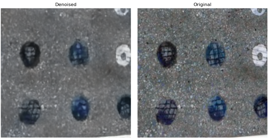
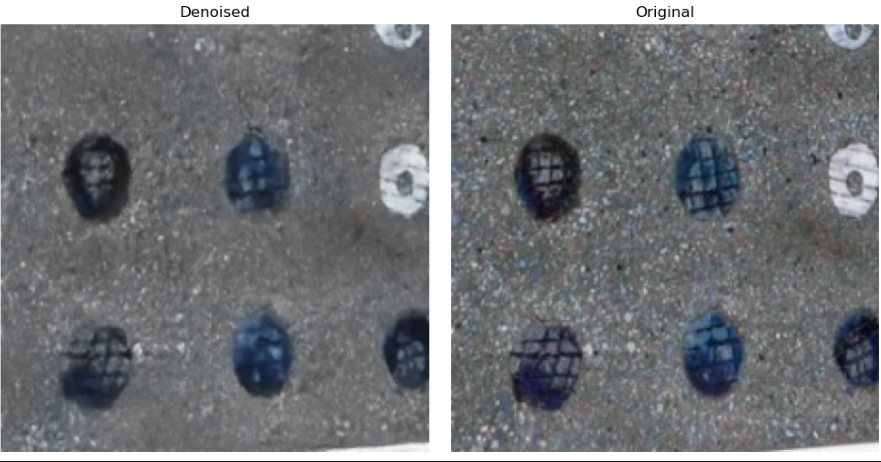
And this one shows the MSE + RegionalSharpnessLoss:

The second one looks much more crisp, doesn’t it? Sadly, it introduces the so-called checkerboard artifact, probably because of the windowing method I used. It may not be visible unless you try very hard to see it, but it’s there. It also causes some weird discoloration in some images. But, like I said - it helped with the annoying blur, hmmm…
At this point, I remembered something from my university days - in my professional career I’ve been a pretty standard web-oriented programmer, so I didn’t really have many opportunities to use any of the advanced math and algorithms I learned. To be honest, I’ve forgotten most of it; maybe that’s why I’m having so much fun rediscovering it while experimenting with AI :)
Anyway, that advanced math/algo I’m referring to is the Fast Fourier Transform. RegionalSharpnessLoss scores sharp pixel intensity changes within windows and compares them between images. You could say it’s a simplistic proxy for what an algorithm based on FFT would do and relating the two is how I arrived at the idea of using the later.
FFT analyzes a signal’s global frequency content. Think of two sinusoids, sin(2x) and sin(4x). Their sum contains components at frequencies 2 and 4; when you sample that sum and run an FFT, the spectrum shows peaks at those frequencies. Peaks - meaning numbers greater than zero. How and why that works is beyond the scope of this blog post, and since I’m not a mathematician, I believe there are people way smarter than me that can explain it. This guy and this guy both give perfect explanations. I said it works globally, but nothing in FFT says it wouldn’t work with rolling windows - as in RegionalSharpnessLoss. No matter how it’s used, it will do the same - it will find the frequencies involved. Also, it’s good to ask what’s the intuition behind a frequency in the context of image processing? Mine was (as confirmed by various language models :) ) that it’s valid to say that sharp difference in pixel values create high frequencies.
I mentioned that a signal relates to a mathematical function, but since FFT only requires sampled data to do its magic, not the function itself, we can pretend the images were created by some function and pass their pixel values as data into one of 999 handy utilities that comes bundled inside pytorch framework - the torch.fft namespace. Before I lay out the full implementation, I’ll use a simple example of how it will work:
import torch
import torchvision.transforms as T


def get_image(thickness: float, blur: str | None = None) -> torch.Tensor:
    H = W = 256
    radius, bg, fg = 60.0, 0.0, 1.0
    y = torch.arange(H, dtype=torch.float32) - H // 2
    x = torch.arange(W, dtype=torch.float32) - W // 2
    Y, X = torch.meshgrid(y, x, indexing='ij')
    dist = torch.hypot(X, Y)
    img = torch.full((H, W), bg, dtype=torch.float32)
    ring = (dist >= radius - thickness / 2) & (dist <= radius + thickness / 2)
    img[ring] = fg

    if blur is None:
        return img

    k, sigma = (5, 1.0) if blur == "less" else (15, 3.0)
    blur_op = T.GaussianBlur(kernel_size=k, sigma=sigma)

    return blur_op(img.unsqueeze(0)).squeeze(0)


def draw_image(img: torch.Tensor, thickness: float) -> None:
    plt.figure(figsize=(6, 6))
    plt.imshow(img.cpu().numpy(), cmap="gray", vmin=0, vmax=1)
    plt.title(f"Gray background with {thickness}px white ring")
    plt.axis('off')
    plt.show()
That function will create a B/W image with a circle in the center. It can either be blurried or not blurried. Let’s generate two images, run fft2 on them and see what were the differences in frequency magnitudes:
img_normal = get_image(8)
magnitudes_normal = torch.fft.fft2(img)
absolute_magnitudes_normal = torch.abs(magnitudes_normal)
img_blur = get_image(8, "more")
magnitudes_blur = torch.fft.fft2(img_blur)
absolute_magnitudes_blur = torch.abs(magnitudes_blur)

(absolute_magnitudes_normal - absolute_magnitudes_blur).abs().mean()
14.8913 - that’s the number that quantifies the differences between the two images. So in a form of a full loss function it will look like this:
class FrequencySharpnessLoss(nn.Module):
    def forward(self, outputs: torch.Tensor, targets: torch.Tensor) -> torch.Tensor:
        out_fft = torch.fft.fft2(outputs)
        tgt_fft = torch.fft.fft2(targets)
        out_mag = out_fft.abs()
        tgt_mag = tgt_fft.abs()
        loss = (out_mag - tgt_mag).abs().mean()
        loss = loss / 1000.0

        return loss
That division by 1000 may look arbitrary, but I did that to put the loss value on the same scale as MSE loss. I again used 0.8, 0.2 weights and the result is again better from the one obtained by the MSE-trained network. See for yourself:
And this one shows the FFT + MSE -trained network result:
The checkerboard has vanished too, but the overal result seems less sharp. Maybe something can be done about it. But before I move on to the final implementation, a word of explanation. The ViT + U-Net model I’m using as a baseline here has been trained with MSE loss function. Then, during the testing phase I also used MSE. But in this post I’m using MSE + another loss function. It’s hard to compare the results in this setup, so I decided to make it simple: I’ll consider a result better, if the related MSE is no greater than that of the baseline model, and visually it looks better. Would that slide in a scientific paper? No. But this is not a scientific paper, so… :)
The code - sharpening the “advanced” way
So there’s one more optimization technique that could be employed here. Does it matter much for this dataset? No. Okay, does it at least make the results visibly better? Sometimes yes, but sometimes they’re slightly worse. Why am I describing it anyway? Well, for one, I spent a good amount of time figuring it out. The other reason is that it may come in handy in some other problems. The optimization technique is: putting more emphasis on high frequencies. I hoped it would make edges sharper, and it did, but not to a degree that would push my baseline MSE even lower.
class FrequencySharpnessLoss(nn.Module):
    def __init__(self, high_freq_weight: float = 2.0):
        super().__init__()
        self.high_freq_weight = float(high_freq_weight)

        self.register_buffer("_freq_mask", None, persistent=False)

    def forward(self, outputs: torch.Tensor, targets: torch.Tensor) -> torch.Tensor:
        _, __, H, W = outputs.shape
        mask = self._ensure_mask(H, W, outputs.device, outputs.dtype)
        out_fft = torch.fft.fftshift(torch.fft.fft2(outputs), dim=(-2, -1))
        tgt_fft = torch.fft.fftshift(torch.fft.fft2(targets), dim=(-2, -1))
        out_mag = out_fft.abs()
        tgt_mag = tgt_fft.abs()
        diff = (out_mag - tgt_mag).abs() * mask
        loss = diff.mean()
        loss = loss / 1000.0

        return loss

    @torch.no_grad()
    def _ensure_mask(self, H: int, W: int, device, dtype) -> torch.Tensor:
        if self._freq_mask is None or self._freq_mask.device != device or self._freq_mask.dtype != dtype:
            y = torch.arange(H, device=device, dtype=dtype) - H // 2
            x = torch.arange(W, device=device, dtype=dtype) - W // 2
            Y, X = torch.meshgrid(y, x, indexing='ij')
            dist = torch.hypot(X, Y)
            max_dist = torch.sqrt(torch.tensor((H // 2) ** 2 + (W // 2) ** 2, device=device, dtype=dtype))
            dist_norm = dist / max_dist
            mask = 1.0 + self.high_freq_weight * dist_norm
            self._freq_mask = mask

        return self._freq_mask
fft2 call would return a tensor where the low frequencies are at the edges and high frequencies at the center. fftshift inverts that. Would this algorithm run just fine without this operation? It would! However, note the _ensure_mask method - that’s the actual reason for incorporating the fftshift invocation. _ensure_mask uses the concept of distance, which is intuitively easy to understand, and because of that, this was the easiest way for me to think about the problem at hand, that’s why I defined it like I did. I hope I’ll manage to clear it out in the next lines.
_ensure_mask builds two 1d tensors first (example with H=W=10) and a meshgrid:
tensor([[-5., -4., -3., -2., -1.,  0.,  1.,  2.,  3.,  4.],
        [-5., -4., -3., -2., -1.,  0.,  1.,  2.,  3.,  4.],
        [-5., -4., -3., -2., -1.,  0.,  1.,  2.,  3.,  4.],
        [-5., -4., -3., -2., -1.,  0.,  1.,  2.,  3.,  4.],
        [-5., -4., -3., -2., -1.,  0.,  1.,  2.,  3.,  4.],
        [-5., -4., -3., -2., -1.,  0.,  1.,  2.,  3.,  4.],
        [-5., -4., -3., -2., -1.,  0.,  1.,  2.,  3.,  4.],
        [-5., -4., -3., -2., -1.,  0.,  1.,  2.,  3.,  4.],
        [-5., -4., -3., -2., -1.,  0.,  1.,  2.,  3.,  4.],
        [-5., -4., -3., -2., -1.,  0.,  1.,  2.,  3.,  4.]])
Side note: the X meshgrid is a transposed version of Y.
Then it creates a distance tensor - distance from the center that represents the differences between the frequencies. After normalizing to [0, 1] range, it creates the mask. Values near the center (low frequencies) get weights close to 1.0, while values at the edges (high frequencies) get weights up to ~3.0 (with default high_freq_weight=2.0). This mask emphasizes high-frequency differences in the loss computation. For the toy example of 10x10 image it looks like this:
0	3.00000	2.81108	2.64924	2.52315	2.44222	2.41421	2.44222	2.52315	2.64924	2.81108
1	2.81108	2.60000	2.41421	2.26491	2.16619	2.13137	2.16619	2.26491	2.41421	2.60000
2	2.64924	2.41421	2.20000	2.01980	1.89443	1.84853	1.89443	2.01980	2.20000	2.41421
3	2.52315	2.26491	2.01980	1.80000	1.63246	1.56569	1.63246	1.80000	2.01980	2.26491
4	2.44222	2.16619	1.89443	1.63246	1.40000	1.28284	1.40000	1.63246	1.89443	2.16619
5	2.41421	2.13137	1.84853	1.56569	1.28284	1.00000	1.28284	1.56569	1.84853	2.13137
6	2.44222	2.16619	1.89443	1.63246	1.40000	1.28284	1.40000	1.63246	1.89443	2.16619
7	2.52315	2.26491	2.01980	1.80000	1.63246	1.56569	1.63246	1.80000	2.01980	2.26491
8	2.64924	2.41421	2.20000	2.01980	1.89443	1.84853	1.89443	2.01980	2.20000	2.41421
9	2.81108	2.60000	2.41421	2.26491	2.16619	2.13137	2.16619	2.26491	2.41421	2.60000
And the results? Again, see for yourself (the last one shows the result produced by network trained with the “advanced” loss function):

I guess those last two images could be used in a contest entitled “find 5 differences”. If you look hard enough, you’ll see them.
Summary
After I finished this post, I had a realization that maybe this could be improved. A long, long time ago, I heard about the so-called wavelet analysis that promises to be a more advanced form of Fourier analysis. Notice that the solution I used only informed us about the existence of certain frequencies, not their placement. So what if I incorporate that into the training? But that’s for the future - I need to learn some more math first…