Denoising autoencoders, Part 1 - basic denoising
The DAE concept was one of the first things I encountered in deep learning that truly captivated me. A quick Google search will reveal countless articles explaining it, so the topic must be thoroughly covered by now, right? Well, most of what I found were superficial guides - authors limited their examples to the MNIST dataset and used small, simple networks composed purely of dense layers. While this works for grasping the basics, this post dives deeper. I’ve found I learn best with medium-to-hard examples, so for this experiment, I chose a dataset I’ve already been exploring: the crack dataset from my still-unfinished crack detection series.
What’s a denoising autoencoder?
In short: it’s a neural network that is capable of reconstructing a clean output from a corrupted input. Putting more words to it: this term is best defined through its use cases. Denoising autoencoders (DAEs), for example, are often used to enhance image quality. Imagine working with a dataset of images plagued by visual artifacts. Traditionally, you might tackle this using a library like OpenCV: first, identify the type of noise present in the dataset, then apply a pre-built function like GaussianBlur (if something resembling gaussian noise is present on the images). While this approach can reduce some artifacts after extensive trial and error, the results are often limited. Denoising autoencoders were developed to achieve better outcomes.
A DAE architecture is - on a high level - very similar across models. There’s the encoder module, the decoder module and a bottleneck placed inbetween them:
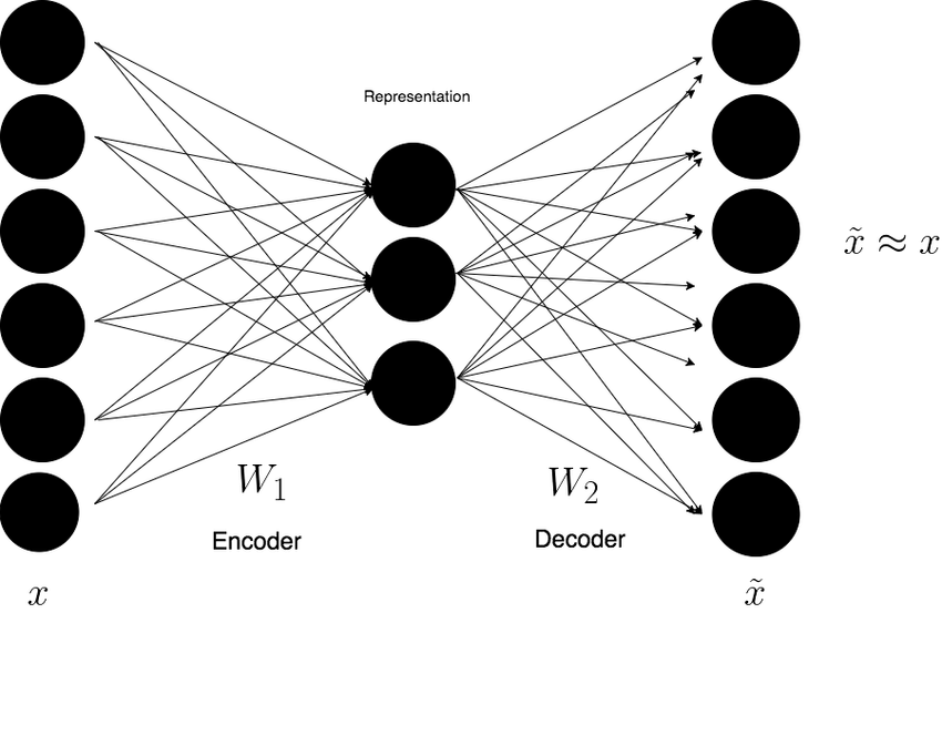 I intentionally chose a diagram that’s highly generic. As you’ll see, even a seemingly simple architecture can take many forms. However, no matter which variant you select, the core architecture remains consistent with the diagram above: an encoder module that compresses the input into a compact bottleneck layer, followed by a decoder module that reconstructs the original data from this compressed representation. The goal of the encoding process is to force the neural network to learn a latent representation - one that retains only the essential features while discarding noise.
The code - baseline
I didn’t want to spend too much time learning “the old way” of denoising, so I used the basic techniques leveraging the OpenCV library:
def calculate_average_mse(original_folder, noised_folder, kernel_size, sigma):
    original_files = [f for f in os.listdir(original_folder) if f.endswith('_raw.jpg')]
    noised_files = [f for f in os.listdir(noised_folder) if f.endswith('_noised.jpg')]
    original_files.sort()
    noised_files.sort()
    mse_list = []

    for original_file, noised_file in zip(original_files, noised_files):
        original_path = os.path.join(str(original_folder), original_file)
        noised_path = os.path.join(str(noised_folder), noised_file)
        original_img = cv2.imread(original_path).astype('float32') / 255.0
        noised_img = cv2.imread(noised_path).astype('float32') / 255.0

        if original_img is None or noised_img is None:
            print(f'Error reading files: {original_file} or {noised_file}')
            continue

        denoised_img = cv2.GaussianBlur(noised_img, kernel_size, sigma)
        mse = mean_squared_error(original_img.flatten(), denoised_img.flatten())
        mse_list.append(mse)

    avg_mse = np.mean(mse_list) if mse_list else float('inf')

    return avg_mse, mse_list


base = Path('/') / 'home' / 'marek' / 'datasets' / 'denoising-nn' / '56x56_tiled'
original_folder = base / 'test'
noised_folder = base / 'test-gaussian'
kernel_sizes = [(3, 3), (5, 5), (7, 7), (9, 9)]
sigmas = [0, 1, 2, 3]
best_mse = float('inf')
best_config = None
mse_lists = None

for kernel_size in kernel_sizes:
    for sigma in sigmas:
        avg_mse, mse_list = calculate_average_mse(original_folder, noised_folder, kernel_size, sigma)

        print(f'Kernel: {kernel_size}, Sigma: {sigma}, Avg MSE: {avg_mse}')

        if avg_mse < best_mse:
            best_mse = avg_mse
            best_config = (kernel_size, sigma)
            mse_lists = mse_list

print(f'Best configuration: Kernel: {best_config[0]}, Sigma: {best_config[1]}, Avg MSE: {best_mse}')
The attached code shows the process of searching for the best-fitting GaussianBlur parameters. Its output is this:
Kernel: (3, 3), Sigma: 0, Avg MSE: 0.00562406936660409
Kernel: (3, 3), Sigma: 1, Avg MSE: 0.005374730098992586
Kernel: (3, 3), Sigma: 2, Avg MSE: 0.00519159808754921
Kernel: (3, 3), Sigma: 3, Avg MSE: 0.0051943715661764145
Kernel: (5, 5), Sigma: 0, Avg MSE: 0.004354353528469801
Kernel: (5, 5), Sigma: 1, Avg MSE: 0.004459990654140711
Kernel: (5, 5), Sigma: 2, Avg MSE: 0.004235366825014353
Kernel: (5, 5), Sigma: 3, Avg MSE: 0.004387643188238144
Kernel: (7, 7), Sigma: 0, Avg MSE: 0.0040468499064445496
Kernel: (7, 7), Sigma: 1, Avg MSE: 0.004397430922836065
Kernel: (7, 7), Sigma: 2, Avg MSE: 0.0043433653190732
Kernel: (7, 7), Sigma: 3, Avg MSE: 0.004775661509484053
Kernel: (9, 9), Sigma: 0, Avg MSE: 0.004193980246782303
Kernel: (9, 9), Sigma: 1, Avg MSE: 0.004395665600895882
Kernel: (9, 9), Sigma: 2, Avg MSE: 0.004441110882908106
Kernel: (9, 9), Sigma: 3, Avg MSE: 0.005127414129674435
Best configuration: Kernel: (7, 7), Sigma: 0, Avg MSE: 0.0040468499064445496
Visual inspection shows that the achieved result is highly unsatisfactory:
GaussianBlur does exactly what its name says: it blurs the image. Maybe with some experimentation this solution could have been made better, but let’s not waste time and move to the first DAE implementation.
The code - basic DAE
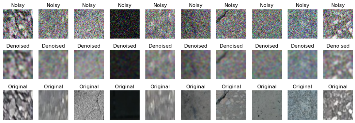
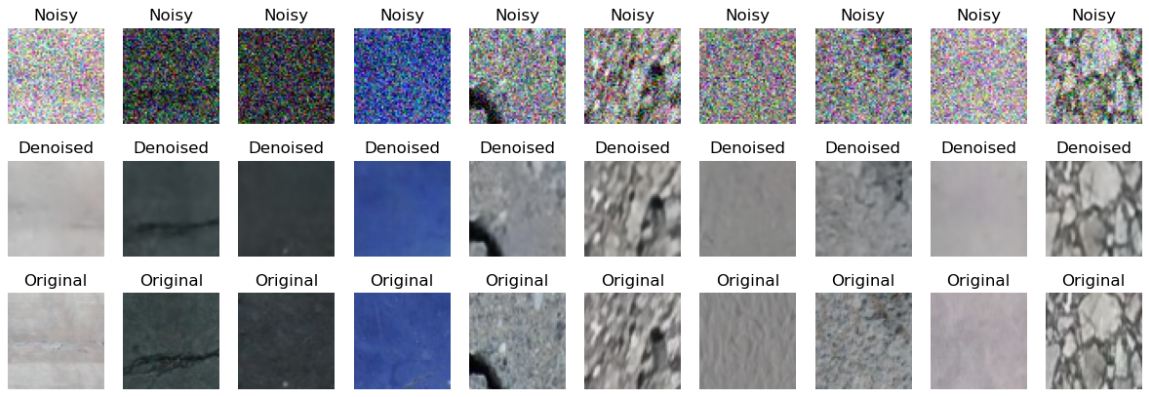
The first model I run was almost 1:1 code I copied from some blog post I found. That’s also why I’m not showing its code - it would be just noise. “Almost” - because my dataset consists of 56x56 images and that blog post was for the MNIST dataset (28x28 images). I also experimented with different layer sizes, but the best result that I achieved was this (with average test MSE across the dataset == 0.0088):
That’s… Pretty underwhelming. However, this screenshot points to something - network is capable of learning something that is currently represented by mostly correct coloring without gaussian blur interference. At that moment I remembered that there exist some widely-known and simple techniques to make networks more capable of learning important features and one of them is using skip connections. Let’s illustrate that with code:
class DAE(nn.Module):
    def __init__(self):
        super(DAE, self).__init__()

        self.input_size = size * size * 3
        self.channel_size = self.input_size // 3
        self.encoder1_out = (self.input_size - int(self.input_size * 0.1)) // 3 * 3

        encoder2_out = self.encoder1_out // 3 - int(self.encoder1_out // 3 * 0.2)
        encoder3_out = self.encoder1_out // 3 - int(self.encoder1_out // 3 * 0.4)

        def create_module():
            return nn.Sequential(
                nn.Linear(self.encoder1_out // 3, encoder2_out),
                nn.ReLU(),
                nn.Linear(encoder2_out, encoder3_out),
                nn.ReLU(),
                nn.Linear(encoder3_out, encoder2_out),
                nn.ReLU(),
                nn.Linear(encoder2_out, self.encoder1_out // 3),
            )

        self.module1 = create_module()
        self.module2 = create_module()
        self.module3 = create_module()
        self.fc1 = nn.Linear(self.input_size, self.encoder1_out)
        self.fc6 = nn.Linear(self.encoder1_out, self.input_size)
        self.relu = nn.ReLU()
        self.sigmoid = nn.Sigmoid()

    def forward(self, x):
        x = x.view(-1, self.input_size)
        encoded = self.relu(self.fc1(x))
        split_size = self.encoder1_out // 3
        x1, x2, x3 = torch.split(encoded, [split_size, split_size, split_size], dim=1)
        x1 = self.module1(x1)
        x2 = self.module2(x2)
        x3 = self.module3(x3)
        decoded = torch.cat((x1, x2, x3), dim=1)
        skip_connection = self.fc6(decoded) + x
        output = self.sigmoid(skip_connection)

        return output.view(-1, 3, size, size)
Side note: you might have noticed that I’m also using 3 modules. The idea here was that perhaps in a dataset like the one I’m using it would be beneficial to try to teach the network to make a 3-channel split. I must confess - I didn’t check the activations, so I can’t tell if it really does that, but I observed that after employing this technique there was a small bug significant performance boost of 0.0005, so I decided to stick with it.
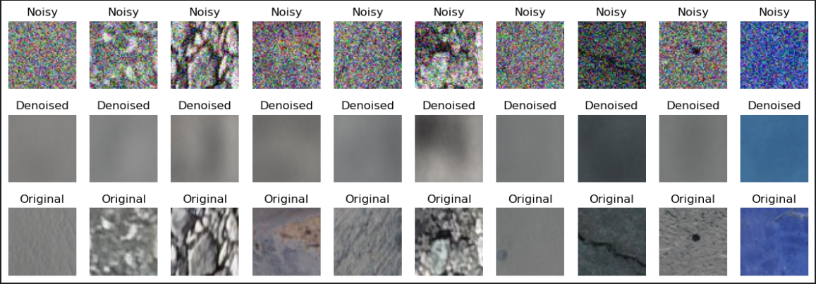
Skip connections don’t alter the core architecture, as they’re only applied within the forward method. The goal here was to combine the flattened raw-input with the final decoder layer. The initial results performed poorly because the latent representation compressed the input too aggressively. A natural question arises: why not increase the bottleneck size? The answer is that doing so risks the network memorizing training patterns, leading to underfitting. But won’t directly adding inputs to the outputs cause overfitting or force the model to memorize noisy data in the final layer? In this case, while it didn’t lead to overfitting, the model began retaining some noise - though it also improved at extracting finer details (with average test MSE across the dataset == 0.0070):
It was a good direction but can this be improved further?
As the final upgrade I decided to use AdamW + Lookahead optimizers combination hoping to squeeze every last bit of accuracy from the model:
criterion = nn.MSELoss()
base_optimizer = optim.AdamW(model.parameters(), lr=0.001, weight_decay=0.01)
optimizer = Lookahead(base_optimizer, k=5, alpha=0.5)
Side note: I didn’t show it in any of the previous snippets, but I’ve been using MSELoss and Adam optimizer so far.
How did I come up with this idea, since using the standard Adam optimizer is such a popular choice? Well, at first I tried sticking with it and improving the model itself, but no changes to the layers or the number of neurons would help. I also tried augmenting the dataset itself with this code, also achieving nothing:
custom_transform = transforms.Compose([
    transforms.ToTensor(),
    transforms.Normalize(mean=dataset_mean, std=dataset_std)
])
When I sampled a few images, most appeared gray (primarily concrete cracks). However, upon closer inspection, a significant portion looked entirely different - some were blue, while others were nearly black. With more data engineering, I could have grouped them and calculated group-specific means and standard deviations. Instead, I shifted angle and started thinking about using another optimizer. I suspected the model underperformed because Adam caused it to settle in local minima, as images within groups were highly similar and some groups dominated the dataset. To expand on that last sentence: Adam is generally less prone to local minima than non-adaptive optimizers (like SGD without momentum) due to its momentum and adaptive learning rates. However, in cases of low gradient diversity (e.g., repetitive/overrepresented patterns), it can converge too quickly to flat regions. That’s basically the case with this dataset. Many images are similar, add on top of that the gaussian noise which also introduces some pattern overrepresentation.
And so I started googling and found out some very interesting information. It turned out that Adam has a flaw built in; let’s get to it.
Adam optimizer is an adaptive algorithm. This article contains a very good and detailed explanation, so I won’t repeat that here. I’ll just outline the main point. This optimizer is adaptive, meaning that it changes the amount by which it updates model’s weights - it adjusts learning rates per-parameter using exponential moving average of gradients (first moment) and exponential moving average of squared gradients (second moment). When gradients are small and consistent, it takes larger steps; when gradients are large or noisy, it takes smaller steps. The first moment is analogous to SGD’s momentum, and the second moment measures the variability of gradients. Another side of Adam is (or rather should be - otherwise there would be no need for the AdamW optimizer) the L2 regularization technique - it’s supposed to push the model to learn smaller weight values, because it was observed that models with smaller weights generalize better. The mentioned flaw makes the L2 step less useful - basically because of a misplaced operation the L2 result is weighed-down. AdamW promises to fix that.
As for the Lookahead meta-optimizer: the problem it Addresses is that standard optimizers can overshoot or oscillate in noisy loss landscapes. A solution proposed by the Lookahead algorithm is to use a set of weights (slow weights) that would act as a “memory” of good parameter regions, reducing sensitivity to short-term gradient noise. Slow weights are calculated by interpolating between the current slow weights and fast weights. What it also means is that the model is updated less frequently.
To sum it all up and put it in the context of the problem at hand: with Adam optimizer I got stuck, AdamW made it better and using AdamW and Lookahead combo was the ultimate solution.
The code - CONV-based DAE
Since I exhausted all the basic dense layers-based options, I moved to a CNN architecture.
class DAE(nn.Module):
    def __init__(self):
        super(DAE, self).__init__()

        self.encoder = nn.Sequential(
            nn.Conv2d(3, 64, kernel_size=3, stride=2, padding=1),
            nn.ReLU(),
            nn.Conv2d(64, 128, kernel_size=3, stride=2, padding=1),
            nn.ReLU(),
        )
        self.bottleneck = nn.Sequential(
            nn.Conv2d(128, 256, kernel_size=3, stride=2, padding=1),
            nn.ReLU(),
            nn.ConvTranspose2d(256, 128, kernel_size=3, stride=2, padding=1, output_padding=1),
            nn.ReLU(),
        )
        self.decoder = nn.Sequential(
            nn.ConvTranspose2d(128, 64, kernel_size=3, stride=2, padding=1, output_padding=1),
            nn.ReLU(),
            nn.ConvTranspose2d(64, 3, kernel_size=3, stride=2, padding=1, output_padding=1),
            nn.Sigmoid()
        )

    def forward(self, x):
        encoded = self.encoder(x)
        bottleneck = self.bottleneck(encoded)
        decoded = self.decoder(bottleneck)

        return decoded
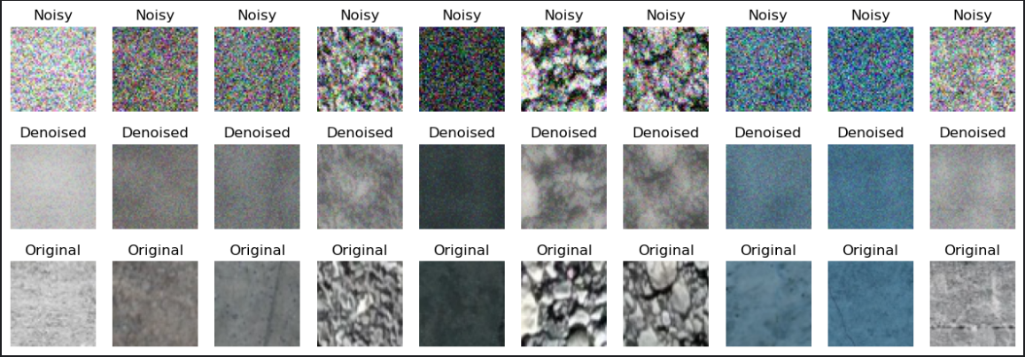
Interestingly, using a skip connection only made the network memorize the noise (test MSE of over 0.03 - an order of magnitute greater than FCN-based network), but using the network in the current form allowed it to achieve test MSE of 0.0017 (vs 0.0070 with FCN net):
The code - UNet
Using a UNet architecture was the natural choice after achieving such a stellar result with basic convolutional network:
class UNetDAE(nn.Module):
    def __init__(self):
        super(UNetDAE, self).__init__()

        self.encoder1 = UNetDAE._conv_block(3, 64)
        self.encoder2 = UNetDAE._conv_block(64, 128)
        self.encoder3 = UNetDAE._conv_block(128, 256)
        self.bottleneck = UNetDAE._conv_block(256, 512)
        self.upconv3 = nn.ConvTranspose2d(512, 256, kernel_size=2, stride=2)
        self.decoder3 = UNetDAE._conv_block(512, 256)
        self.upconv2 = nn.ConvTranspose2d(256, 128, kernel_size=2, stride=2)
        self.decoder2 = UNetDAE._conv_block(256, 128)
        self.upconv1 = nn.ConvTranspose2d(128, 64, kernel_size=2, stride=2)
        self.decoder1 = UNetDAE._conv_block(128, 64)
        self.output_layer = nn.Conv2d(64, 3, kernel_size=1)
        self.pool = nn.MaxPool2d(kernel_size=2, stride=2)

    def forward(self, x):
        e1 = self.encoder1(x)
        p1 = self.pool(e1)
        e2 = self.encoder2(p1)
        p2 = self.pool(e2)
        e3 = self.encoder3(p2)
        p3 = self.pool(e3)
        b = self.bottleneck(p3)
        up3 = self.upconv3(b)
        d3 = self.decoder3(torch.cat([up3, e3], dim=1))
        up2 = self.upconv2(d3)
        d2 = self.decoder2(torch.cat([up2, e2], dim=1))
        up1 = self.upconv1(d2)
        d1 = self.decoder1(torch.cat([up1, e1], dim=1))

        return self.output_layer(d1)

    @staticmethod
    def _conv_block(in_channels, out_channels):
        return nn.Sequential(
            nn.Conv2d(in_channels, out_channels, kernel_size=3, stride=1, padding=1),
            nn.ReLU(inplace=True),
            nn.Conv2d(out_channels, out_channels, kernel_size=3, stride=1, padding=1),
            nn.ReLU(inplace=True)
        )
You may be asking why did using something resembling skip connections worked for this UNet’s implementation while doing it slightly differently in a non-UNet architecture completely derailed the training. The devil is in the details. In my implementation I just added the x tensor to the decoder’s output, like this:
def forward(self, x):
    skip = x
    encoded = self.encoder(x)
    bottleneck = self.bottleneck(encoded)
    decoded = self.decoder(bottleneck)
    output = decoded + skip
    output = self.sigmoid(output)

    return output
Convolutional layers are extracting features way better than the fully connected ones, so adding the raw input signal in only disrupts the output. While the first model was pretty lame at extracting those features on its own, adding the skip connection made it better but still pretty lame overall. However, convolutions did pretty great on their own - hence the disruption. But maybe something similar could have been utilized? That’s the question I asked myself and that’s how I arrived at the idea of using a UNet architecture.
The general idea resembled skip connections, but instead of adding in the raw signal to the top of the network, it adds the feature information after it gets extracted by encoder modules (and does it 3 times). This way the decoder module gets pushed into the right direction - it receives progressively cleaner information which it leverages to make the reconstruction better.
The top result I achieved with UNet was somewhere between 0.0016 and 0.0015. I won’t attach the images, because visually it’s close to impossible to tell the difference between the UNet’s result and the result achieved by the basic conv net.
Summary
Even though I did put “Part 1” into this article’s title, I’m not sure if I’ll find time to dig more into this topic. But if I do, I’ll try looking for something to make the UNet solution even better. I read that this kind of architecture is used for generating super-resolution images, so I’ll search for methods of doing that and getting test MSE even below 0.001 treshold.