Comparing models using SmoothL1Loss and CIoU loss functions
The two previous articles focused on two very similar models. One was trained using the SmoothL1Loss function, and the other using the CIoU loss function. Additionally, there was a third model not covered by any of the articles. Its architecture was the same as the one using CIoU loss, but it was trained using SmoothL1Loss.
The justification
Each of the trained variations was run 20 times. This means that the checkpoints directory, where their weights were saved, needs to be iterated over to find the most performant one. While this is not the most optimal method - since a better model for a given variation could have been saved with an accuracy value for comparison - I was also interested in conducting a short statistical analysis of the models, specifically, how spread out their results are. The value of this information is to help inform next steps.
In a “real world” scenario, some model architecture might perform best for a given dataset. Over time, you may notice that the results for certain types of images are noticeably worse than the results for the rest of the images. As more data comes in, you may want to retrain your models. One way to optimize time use would be to pick the N most accurate models, but this might result in the same outcome. However, if you can determine which architectures give the most consistent results when retrained, it would help in making a more informed decision. In the worst case, the second choice might not be the most accurate one, but at least you can be confident that its results won’t vary significantly.
As for the statistical analysis - I will probably post it as a separate blog post later.
The code
The basic setup contains two models architectures and a dictionary of arrays of results for each.
variations = {
    "1": BasicBoundingBoxModel,
    "2": BiggerBasicBoundingBoxModel, # this one was trained using SmoothL1Loss
    "3": BiggerBasicBoundingBoxModel  # and this one was trained using CIoU loss
}
model_metrics = {
    "1": [],
    "2": [],
    "3": []
}
The code snippet below loads every checkpoint and runs it against the test dataset. One interesting thing to note is that each metric row is a tuple of two values. The first value is the SmoothL1Loss, and the second is the CIoU loss. I structured it this way because I was curious to see how well a model trained with one loss function would perform when evaluated with the other.
with torch.no_grad():
    for filename in os.listdir("checkpoints"):
        if filename.endswith(".pt"):
            parts = filename.split("_")
            model_variation = parts[1]
            run_index = parts[5].split(".")[0]
            model_path = os.path.join("checkpoints", filename)
            model = variations[model_variation]().to(device)
            smooth_l1_loss_f = nn.SmoothL1Loss()
            ciou_loss_f = CIoULoss()

            model.load_state_dict(torch.load(model_path, map_location=device))

            metrics = []

            for data in test_loader:
                inputs, true_boxes = data
                true_boxes = torch.stack(extract_bboxes(true_boxes)).to(device)
                inputs = inputs.to(device)
                pred_boxes = model(inputs)
                l1_metric = smooth_l1_loss_f(pred_boxes, true_boxes)
                ciou_loss = ciou_loss_f(pred_boxes, true_boxes)

                metrics.append((l1_metric, ciou_loss))

            mean_l1_metric = sum(map(lambda x: x[0], metrics)) / len(metrics)
            mean_ciou_metric = sum(map(lambda x: x[1], metrics)) / len(metrics)

            model_metrics[model_variation].append((mean_l1_metric, mean_ciou_metric))
This code selects the best variations.
best_variations = {
    "1": [],
    "2": [],
    "3": []
}

for namespaced_key, tensors in model_metrics.items():
    l1_items = list(map(lambda x: x[0].item(), tensors))
    ciou_items = list(map(lambda x: x[1].item(), tensors))
    min_l1 = min(l1_items)
    min_ciou = min(ciou_items)
    min_l1_idx = l1_items.index(min_l1)
    min_ciou_idx = ciou_items.index(min_ciou)
    variation_number_l1 = min_l1_idx + 1
    variation_number_ciou = min_ciou_idx + 1

    best_variations[namespaced_key].append({
        f"{str(variation_number_l1)}_l1": min_l1,
        f"{str(variation_number_ciou)}_ciou": min_ciou
    })
The contents of the best_variations variable looks like this:
{'1': [{'18_ciou': 0.23365730047225952, '6_l1': 5.894285678863525}], '2': [{'4_ciou': 0.22702017426490784, '4_l1': 5.780552387237549}], '3': [{'18_l1': 6.124795913696289, '9_ciou': 0.23207801580429077}]}
It’s clear that the variation that won is the second one. Not only did it achieve the lowest error rate for the SmoothL1Loss, but also for the CIoU loss. It also seems that for this problem and architecture(s), the use of CIoU loss was not the best choice.
It’s always good to visualize the results which is done in the next snippet:
def draw_rectangle(
        orig: PIL.Image.Image,
        coords: tuple[int, int, int, int],
        new_path: str,
        rect_color='red',
        rect_width=1) -> None:
    copy = orig.copy()
    draw = ImageDraw.Draw(copy)

    draw.rectangle(coords, outline=rect_color, width=rect_width)
    copy.save(new_path)


with torch.no_grad():
    for idx, (images, targets) in enumerate(test_loader_small_batch):
        images = images.to(device)
        outputs = model(images)
        img_id = dataset.ids[idx]
        img_info = dataset.coco.loadImgs(img_id)[0]
        img_path = img_info["file_name"]
        orig_img = PIL.Image.open(os.path.join(root, img_path))

        for output in outputs:
            coords = tuple(map(int, output[:4]))
            output_path = os.path.join(out_dir, os.path.basename(img_path))
            draw_rectangle(orig_img, coords, output_path)


Summary
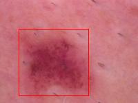
I attached six images: three are lesion images with predicted bounding boxes overlaid on top, and the other three are segmentation masks used to create the COCO file containing the x and y coordinates of the ground truth bounding boxes. Two of the models accurately predicted lesion locations, but one did not. If you look at the related segmentation mask, it seems it should locate a lesion close to the bottom-left corner of the image, but instead, it spanned almost to the top right corner. Why is that? On the attached lesion image, it’s clear that there are actually two darker spots. This tells us two things:
The presence of the other black spot confused the model. The model seems to “understand” that a lesion is usually different in color from the rest of the image, which is why it tries to box the second dark image element as well. This partially explains why such a simple architecture was able to achieve such low error rates - the task was relatively simple.