Attention mechanisms explained… Again!
While still experimenting with the ancient R-CNN architecture, I find myself exploring different territories - mainly because of the long wait times while models finish training. This time, my thoughts drifted toward the transformer architecture. It might seem funny, given that the whole world seems to understand and use it already - and so did I - until I realized I don’t fully grasp the attention mechanism at its core. That’s a problem since attention is the essence of transformers.
It’s been a long time since I last crammed transformer knowledge into my brain, and much of it has faded over time. So, since explaining concepts is one of the best ways to reinforce and deepen understanding, I’ll attempt to do just that in this post.
The code, the math
In his short book Helgoland, Carlo Rovelli writes (not a direct quote) “it’s all in the relations”. Elements of matter don’t possess intrinsic properties on their own; rather, they exhibit certain properties through interactions with other elements of matter. Reality is relational, and to a big extent, the same applies to language, as the transformer architecture demonstrates.
The first component of the transformer encoder module is the embedding layer combined with positional encoding. Explaining these in detail isn’t the goal of this post, but I’ll try to cover them using my understanding. Let’s assume a sentence has passed through this initial layer and is now represented by six vectors:
v1 = np.array([1, 0, 0])
v2 = np.array([0.95, 0.1, 0])
v3 = np.array([0, 1, 0])
v4 = np.array([0, 0.95, 0.1])
v5 = np.array([-1, 0, 0])
v6 = np.array([0.5, 0.5, 0.5])
semantic_vectors = np.array([v1, v2, v3, v4, v5, v6])
If you plot them, you’ll see that some of them align with others better than the rest:
semantic_labels = ["v1", "v2", "v3", "v4", "v5", "v6"]
semantic_colors = ["r", "r", "b", "b", "g", "orange"]

%matplotlib notebook
fig = plt.figure(figsize=(14, 6))
ax1 = fig.add_subplot(121, projection="3d")

for i in range(len(semantic_vectors)):
    ax1.quiver(
        0,
        0,
        0,
        semantic_vectors[i][0],
        semantic_vectors[i][1],
        semantic_vectors[i][2],
        color=semantic_colors[i],
        label=semantic_labels[i]
    )

ax1.set_xlim([-1.5, 1.5])
ax1.set_ylim([-1.5, 1.5])
ax1.set_zlim([-1.5, 1.5])
ax1.set_title("Semantic Vectors")
ax1.legend()
plt.tight_layout()
plt.show()
Side note: I might as well used 2d vector representations, but I needed some fanciness in my life and adding another dimensions doesn’t make this problem harder to understand.
The two blue ones point mostly in the same direction, as do the red ones. The yellow one is somewhere inbetween and the green one points to the direction oposite to the red ones, and is orthogonal to the blue ones:
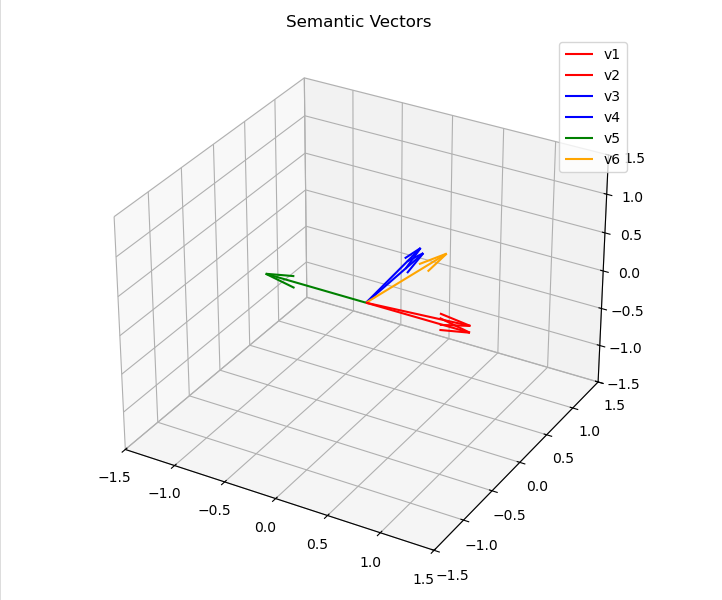
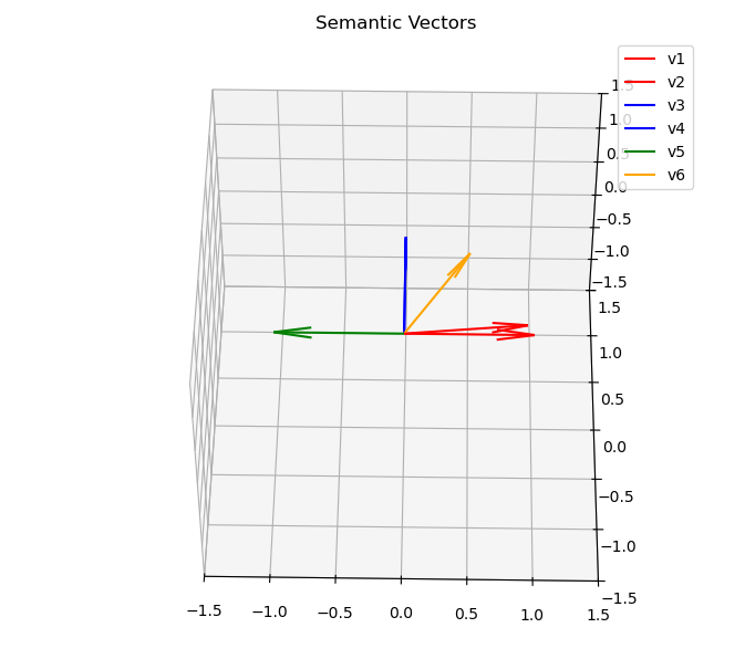
Think: semantic meaning. The vectors in blue and red pairs may be sharing meaning (vector to vector, not pair to pair), like: (v1, v2) = (dog, puppy) and (v3, v4) = (forest, tree). The v6, yellow vector, is supposed to be kind of a “bridge” - something that holds meaning common to the two pairs, but I can’t come up with any word to illustrate that :) The v5 vector is supposed to be the oposite to the red ones - I’m also unable to come up with a good example, but I think this setup is so easy to understand that examples are not really necessary. All those relations can be mathematically described with cosine similarity function - it will be used later.
The semantic meaning is obtained, but the transformer architecture also uses positional information and the authors of the original paper encode that with function similar to this one:
def positional_encoding(position: int, d_model: int) -> np.ndarray:
    PE = np.zeros((position, d_model))

    for pos in range(position):
        for i in range(0, d_model, 2):
            PE[pos, i] = np.sin(pos / (10000 ** (i / d_model)))

            if i + 1 < d_model:
                PE[pos, i + 1] = np.cos(pos / (10000 ** ((i + 1) / d_model)))

    return PE
I also define two helper functions:
def cosine_similarity(vec1, vec2):
    return np.dot(vec1, vec2) / (np.linalg.norm(vec1) * np.linalg.norm(vec2))


def get_similarities(vectors: np.ndarray):
    similarity_results = {}

    for i, j in combinations(range(6), 2):
        pair = f"v{i + 1} and v{j + 1}"
        similarity_results[pair] = cosine_similarity(
            vectors[i],
            vectors[j]
        )

    print("Cosine Similarity between vector pairs:")

    for pair, similarity in similarity_results.items():
        print(f"{pair}: {similarity:.2f}")
I initially treated positional encodings as a technical detail that helps transformers perform better and I never really questioned why the function is defined the way it is. When I started Googling and ChatGPT-ing for answers, every explanation seemed to deepen my confusion. I began to suspect that I may be missing the mathematical intuition needed to analyze this like a pro. So, being as lazy as I am, I opted for an empirical approach. I asked myself two questions:
- Why can’t either sine or cosine function be used? Why use both?
- Can I come up with another function that would encode positional information like this one does?
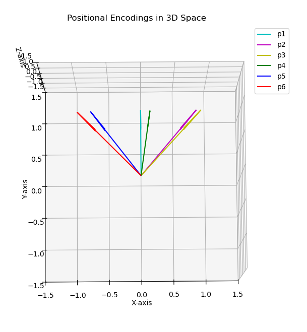
The first question can be explained easily if you make the step range function argument equal to 2 and you comment out the if statement. This is the result:

There are three pairs, and vectors in each of them overlap so it seems they don’t encode positional information very well. However, when the positional_encoding function is used in the form I posted here, it gets better:
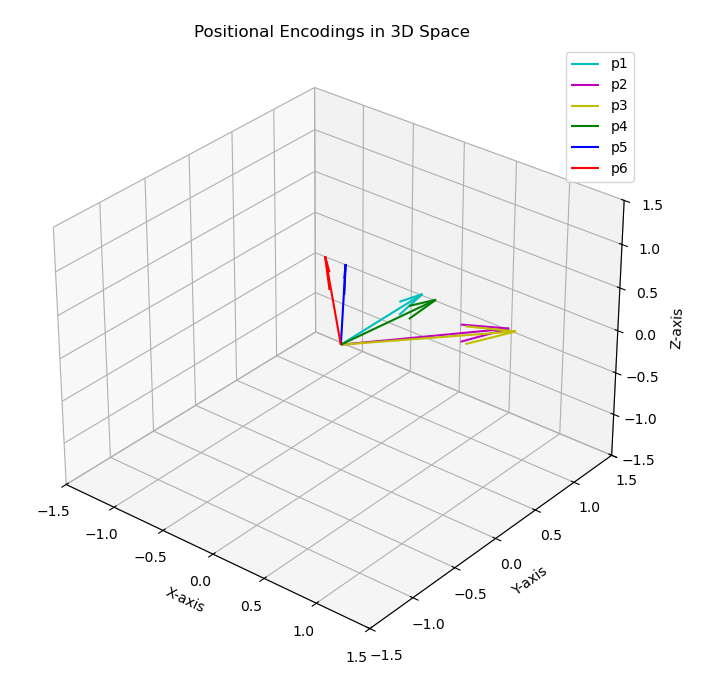
They still overlap to some extent. However, note that they got closer together (and the orthogonality of the green vector with the two pairs vanished). To check how this looks like in 512 dimensions I just run the get_similarities function for positional encodings generated for 512 dimensions. Then I did the same for 3d vectors and these are the cosine similarity results between each pair of vectors:
Cosine Similarity between vector pairs (3d):
v1 and v2: 0.76
v1 and v3: 0.74
v1 and v4: 0.99
v1 and v5: 0.79
v1 and v6: 0.71
v2 and v3: 1.00
v2 and v4: 0.85
v2 and v5: 0.21
v2 and v6: 0.09
v3 and v4: 0.83
v3 and v5: 0.17
v3 and v6: 0.05
v4 and v5: 0.70
v4 and v6: 0.61
v5 and v6: 0.99

Cosine Similarity between vector pairs (512d):
v1 and v2: 0.97
v1 and v3: 0.91
v1 and v4: 0.83
v1 and v5: 0.77
v1 and v6: 0.74
v2 and v3: 0.97
v2 and v4: 0.91
v2 and v5: 0.83
v2 and v6: 0.77
v3 and v4: 0.97
v3 and v5: 0.91
v3 and v6: 0.83
v4 and v5: 0.97
v4 and v6: 0.91
v5 and v6: 0.97
In higher dimensions, positional information becomes more clustered but no two vectors are perfectly aligned (like v2 and v3: 1.00 in the lower-dimensional example), and lacks abrupt jumps. Stability is a quality most AI architecture designers strive for, and this method of positional encoding seems to provide consistently stable values.
As for the second question (“Can I come up with another function that would encode positional information like this one does?”) - there are likely many possible functions, but I lack the mathematical tools to identify them. So, my answer is no :) However, one idea I considered was dividing the word’s position number (e.g., 1, 2, etc.) by the dimensionality value (e.g., 1/512, 2/512) and then adding that fraction to each dimension. However, this approach would result in a linear function, which might not be desirable here. Additionally, the values would become unevenly distributed at the edges of the range: tiny for the early words and excessively large at the end. In an extreme scenario with a sequence of 512 tokens, the final token would require adding 1 (one) to each dimension.
In contrast, the sine and cosine combination offers a much more constrained and stable representation. That said, this is merely a hypothesis - I’m aware it’s more hand-waving than a rigorous explanation.
Let’s take another step. The embeddings are ready and the positional encodings are ready as well. The transformer architecture adds them to obtain the vectors that will be passed into the attention mechanism. I could attach a screenshot of the vectors after adding them, but that wouldn’t provide any insight. It suffices to say that the vectors change, but that’s kind of obvious :)
Enter: attention mechanism. The algorithm is as follows:
- Matrices \(Q\) and \(K^T\) are multiplied to form the so called attention scores - the multiplication result represents how important each token is to another token.
- Their values are scaled down by dividing them by \(\sqrt{d_k}\) (the dimensionality of each query and key vector).
- That’s done in case the dot products created in the first step are very large (or small) - that could make the softmax function return skewed probability values and also the gradients would be very small.
- Finally, the result of the third step is multiplied by the value matrix \(V\).
The full equation is as follows:
\[\begin{aligned} \text{softmax} (\frac{QK^T}{\sqrt{d_k}})V \end{aligned}\]An obvious question to ask is: what are these matrices, where do they come from? Well, as almost everything in AI, they are learned. In short, the Query ( \(Q\)), Key (\(K\)), and Value (\(V\)) matrices are derived from the input vectors using learned weight matrices. These weight matrices (\(W_Q\), \(W_K\), \(W_V\)) are the ones being adjusted during training, while \(Q\), \(K\) and \(V\) are their projections on these weight spaces (projections made by using a dot product on them and attention layer inputs). I saw the best intuitive explanation about them here. I’ll expand on it adding just a few words to the \(K\) matrix explanation. Think of the \(K\) matrix as representing “keywords” or “matching criteria” that other tokens will use to determine relevance. While the \(V\) matrix holds the content payload, the \(K\) matrix acts like a filter or signature that determines how well a token aligns with a Query. Let’s use an example sentence: “The cat sat on a mat and spilled milk over it”. So, when you state the problem the way mr. Juan Olano does, it seems that the goal of attention mechanism is to obtain input vector representations that would add those three dimensions:
- What is a given token asking for? A brutal simplification would be that if token \(x_1\) represents the word “it”, then the \(Q\) matrix encodes what “it” is looking for in the surrounding context - connections to related meanings, like “cat”, “mat” etc.
- Which other tokens (meanings) match - that’s the \(K\) matrix; It represents how strongly each token aligns with what “it” is searching for.
- What actual content does this token have to share if it’s found relevant? That’s the \(V\) matrix. Once the alignment has been established (via Query and Key), the token’s Value contributes its semantic content.
In the beginning these three points sounded very similar to each other to me. That’s because all of those three matrices basically deal with semantic meaning, but sometimes the way to understanding is just finding a good example: if “it” focuses on “milk”, then the Value vector from “milk” might include information like “a liquid, related to spilling”.
Now let’s put all that into code. Obviously, I won’t be recreating the actual iterations Transformers perform to arrive at certain \(Q\), \(K\) and \(V\) matrices; instead I’ll simulate the data so that the result matches with the goal Transformers promise to achieve.
W_Q = np.array([
    [1, 0, 0],
    [1, 0, 0],
    [0, 0, 1],
    [0, 0, 0],
    [0, 0, 0],
    [2, 0, 0],
]).T
W_K = np.array([
    [1, 0, 0],
    [1, 0, 0],
    [0, 0, 5],
    [0, 0, 3],
    [0, 0, 5],
    [2, 0, 0],
]).T
W_V = np.identity(3)
Side note: I defined the \(W_V\) as an identity matrix for simplicity, normally it would have its own unique set of values.
The above defines the weight matrices. Don’t focus on the values I used because they are random. Just remember the goal which is transforming the attention layer input so that it represents the contextual information. In terms of math that may mean that the cosine similarity of two contextually related vectors will tend to get closer to 1. However, this doesn’t always happen - if two tokens have multiple competing relationships (ambiguity in a sequence structure, their attentions might diverge).
Having said that, let’s go back to the code:
Q = semantic_vectors @ W_Q
K = semantic_vectors @ W_K
V = semantic_vectors @ W_V
d_k = Q.shape[1]
attention_scores = Q @ K.T / np.sqrt(d_k)
attention_weights = np.exp(attention_scores) / np.sum(np.exp(attention_scores), axis=1, keepdims=True)
attention_output = attention_weights @ V
attention_output_normalized = attention_output / np.linalg.norm(attention_output, axis=1, keepdims=True)
Side note: there’s one fun nuance lurking between these lines which is the attention_scores matrix. Think of it this way: each row in that matrix acts as a set of coefficients that will weight the rows of the value matrix. “What actual content does this token have to share if it’s found relevant?”. Well, the highly weighed rows is the actual content we were asking about.
The last line - normalization - isn’t really required, I only did it to have a nicer plot. Ok, like I said, the matrices were just some dummy data examples, but what would actually happen if the attention mechanism was run for several iterations (at least in the simple case), would be that the cosine similarity of some related vectors would converge. I can simulate that with rotation matrices:
def rotate_n_deg_around_x(v: np.ndarray, n_deg: int) -> np.ndarray:
    theta = np.radians(n_deg)
    R_x = np.array([
        [1, 0, 0],
        [0, np.cos(theta), -np.sin(theta)],
        [0, np.sin(theta), np.cos(theta)]
    ])

    return R_x @ v


def rotate_n_deg_around_y(v: np.ndarray, n_deg: int) -> np.ndarray:
    theta = np.radians(n_deg)
    R_y = np.array([
        [np.cos(theta), 0, np.sin(theta)],
        [0, 1, 0],
        [-np.sin(theta), 0, np.cos(theta)]
    ])

    return R_y @ v
Let’s use these functions on the attention outputs and plot the result:
attention_output_normalized[2] = rotate_n_deg_around_y(
    rotate_n_deg_around_x(attention_output_normalized[2], -75),
    45
)
attention_output_normalized[3] = rotate_n_deg_around_y(
    rotate_n_deg_around_x(attention_output_normalized[3], -80),
    45
)

fig = plt.figure(figsize=(14, 6))
ax = fig.add_subplot(121, projection="3d")

for i in range(len(attention_output_normalized)):
    ax.quiver(
        0,
        0,
        0,
        attention_output_normalized[i][0],
        attention_output_normalized[i][1],
        attention_output_normalized[i][2],
        color=semantic_colors[i],
        label=semantic_labels[i]
    )

ax.set_xlim([-1.5, 1.5])
ax.set_ylim([-1.5, 1.5])
ax.set_zlim([-1.5, 1.5])
ax.set_title("Attention-Modified Token Representations")
ax.legend()
plt.tight_layout()
plt.show()
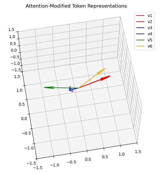
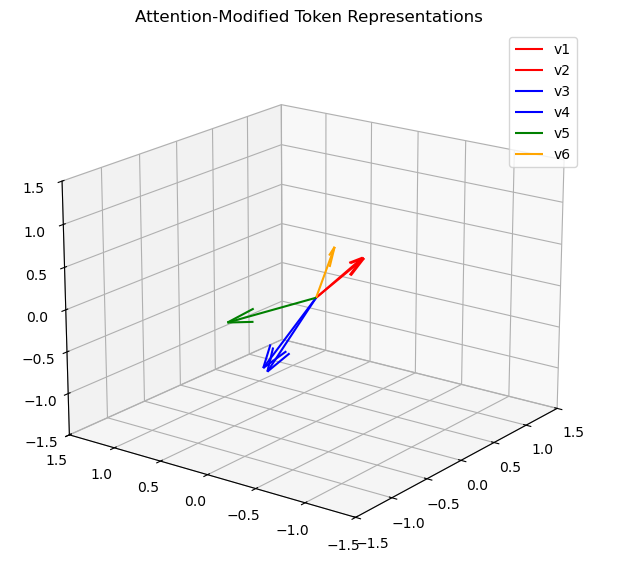
These two perspectives show that v6 has been found to be contextually correlated with v1 and v2 (which are still contextually correlated anyway) and contextually decorrelated from v3 and v4. Obviously, this is just an oversimplified projection that I wrote to understand the purpose of each part. In a real transformer model, or better yet, something as big as ChatGPT, it’s not as straightforward. It takes many iterations and an incredibly large dataset to actually get the correct contextual meaning as shown in the last example with rotations.
Summary
I didn’t cover many other components. After the attention mechanism is applied, the resulting submatrices are concatenated and passed through a layer that incorporates information from a residual connection and normalizes the resulting vectors. Additionally, multiple attention heads run in parallel, collectively forming the step described in this blog post.
However, none of these details were my focus - I simply wanted to understand the mechanics of the attention mechanism. When I started learning to code some 20 years ago, the books about languages like Java or C# were saying “everything is an object” every second page. That’s where I get this projection for attention mechanism: “everything is a dot product”. Not really, because there’s a ton of nuance here, but if you dumb it down, you’ll see that on the mechanistic level, it’s 80% dot product magic :)