Building a tree-based model training pipeline with scoring
In my previous post I mentioned that I have been involved in algotrading software that is supposed to predict price movements in the stock market. Despite what I’ve seen some people say on the internet, it’s not an effort completely doomed to fail.
#1 Obviously, if it were easy, everyone would already be doing it, and I’ve stepped on metaphorical LEGO bricks more than 99,999 times so far, but I also managed to discover that there are things in algotrading that work surprisingly well.
#2 Obviously, the degree of your success will also be heavily dependent on the quality and amount of data that you use - writing web scrapers, if you don’t want to pay for a commercially available API, is another huge subdomain in algotrading.
#3 Maybe less obviously, but still - finding the correct target for your models can also be a huge effort, and defining it as simply as “I will short like crazy, so give me 10,000 tickers that are about to implode tomorrow, so I can sell a truckload of outrageously overpriced calls and pretend margin requirements are just a social construct” won’t work and will make you lose your house, your wife, dog, and kids. Don’t try this at home!
#4 obviously I won’t share the details about what features I use, or other technicalities, because if you do the same, my strategy may stop working! :)
Requirements
Requirements can be laid out simply as building an ML training pipeline that will find the best types/sets of types/hierarchies of models. Before I even started working on this specific piece, I experimented quite a lot in Jupyter Notebooks, exploring how far I could get with XGBoost, LightGBM, and CatBoost on their own. Then I figured out that ensemble methods might work better, since all three are similar in spirit but different in implementation, and perhaps they make different mistakes.
And then, when I saw that my results were basically shit, I sat down and thought even more to find a better target variable. When I came up with one (let’s say it was simply 0 for the price going down the next day vs. 1 for it going up) and experimented some more, it became clear that I needed a two-stage model. One (or an ensemble) would aim for a decent 70% recall at 30% precision, while the second one would optimize only for precision.
I also used the stacking technique, where a meta-model at the end learns how to assess the three models’ predictions if an ensemble has been used; however, it has yet to give me a substantial boost in performance. It’s still a work in progress, so I’ll just describe it as it is now.
Why those specific models?
Well, you might have already noticed that I’m a neural network nerd, so why would I even look at gradient boosting on decision trees techniques, right? I’m pretty sure there are some rich people out there, owning IT companies that hire people way smarter than me have figured out how to train neural nets on stock market data. But me - I haven’t. I tried but my results were so horrible that I would be better off just flipping a coin.
Then I did my research and saw that a lot of people in the quant/algotrading space use XGBoost for their work. Perhaps they are as secretive as I am and they use a lot more (maybe even neural nets or witchcraft, who knows!), but the most prevalent information that I managed to find was screaming XGB at me. You could say that the internet terrorized me into using gradient boosting in this project.
Side note: I was also thinking for a second about using sklearn, but since they don’t support GPU training it wasn’t a viable candidate.
What are the differences?
As it goes for ML, when you see similar libraries, the differences between them are usually very technical and nuanced, and it’s no different this time, so I won’t really go into the details. The thing is, those details usually don’t matter much when you apply the techniques. With dataset A, you’ll get great results with XGBoost. With a similar but slightly different dataset B, you’ll get better results using either of the other two, and so on. So how do I find the best model for my dataset? I run Optuna over a rich search space until it finds something that meets the requirements. Everybody does it :)
But let’s lay out at least some minimal technical details. It is said that XGBoost heavily regularizes its trees to avoid overfitting, and it builds them level-wise, which means it builds all the nodes on a given level before moving on. In other words, it tries to find all the splits on one level, thus avoiding missing something important. XGB trees are more balanced, possibly less deep. LightGBM, on the other hand, builds its trees leaf-wise which means that on each iteration it picks a leaf with the greatest gain and it only splits on that one. Thus, LGBM trees may be unbalanced and very deep. It’s also said this often leads to faster training and better overall results. But in my case, it didn’t train faster, nor did it lead to great results. In my case the standalone LightGBM loses most of the time when pitted against XGBoost or CatBoost; however, it still manages to bring some value to the table. As for CatBoost - I just needed a third model that would serve as a tie breaker. Turns out, I kept losing some predictions in ensemble methods, because XGB and LGBM were not agreeing quite often and it got better after mixing in the third model.
Side note: ok, first and foremost I’m a curious programmer, so I couldn’t leave out one technical detail I only hinted at above: the regularization and tree balancing. So the thing is that XGB implements L1 and L2 regularization in its classic form and it’s used on the level of a tree. You can use these params for regularization:
lambda (L2)alpha (L1)gamma (min split loss)min_child_weightmax_depth
L1 regularization is turned off by default and L2 is turned on. What it all leads to is: XGB trees are often more balanced than LGBM trees. XGB may decide not to split on leaf A, while it still splits on leaf B, but in general it will happen less often than in the case of LGBM. This behavior is an artifact of the architectures both use.
LGBM mostly uses the same regularization math, however it calls some params differently, and also adds some of its own:
lambda_l1lambda_l2min_data_in_leafmin_gain_to_splitmax_depthnum_leaves
L1 and L2 are turned off by default. The min_gain_to_split plays a role that is similar to XGBoost’s gamma - if the value is too low, there’s no split, however, it’s also turned off by default. Also, since it builds its trees leaf-wise, regularization relies more on architectural constraints by default - you can set the num_leaves and min_data_in_leaf params exactly for that, but even if you switch on all the regularization knobs, you’ll be getting less balanced trees most of the time.
But how do these two algorithms even decide whether or not to split (XGB) or where to split (LGBM). They both use the gain metric for that. That’s also another big and important difference between the two. I can summarize it like this: XGB uses the gain metric to limit the splits while LGBM uses the same metric to find the best leaf (the one with the highest gain) to split on.
Anyway, the end effect is that an LGBM tree may look like this:
        [root]
       /      \
     [A]      [B]
    /   \
  [C]   [D]
         |
        [E]
…and XGB tree can look more like this:
        [root]
       /      \
     [A]      [B]
    /   \    /   \
  [C]  [D] [E]  [F]
As for CatBoost and its tree building approach: it uses a strategy called “symmetric trees” (or “oblivious trees”) by default. This means that at each level of the tree, the same split condition is used for all nodes. Sounds limiting, but it leads to very fast inference and acts as a natural form of regularization:
        [age > 30?]
        /         \
   [yes]          [no]
   /    \         /   \
 [inc>50k?]     [inc>50k?] <- same split across the entire level
Looking at the graph, it looks kind of similar to the one for XGB; however, the difference is in the split condition.
As for regularization, CatBoost offers a similar set of parameters:
l2_leaf_reg(equivalent to lambda/lambda_l2)min_data_in_leafmax_depth(defaults to 6, same as XGBoost)num_trees
There’s no direct equivalent of gamma/min_gain_to_split. Instead, CatBoost relies more on symmetric trees and a technique called “ordered boosting”, which prevents prediction shift (a type of overfitting specific to gradient boosting).
One more thing worth noting: CatBoost defaults to grow_policy='SymmetricTree', but you can switch to Depthwise (like XGBoost) or Lossguide (like LightGBM). So technically you can get the behavior of all three libraries in one, it’s just the default setting that differs.
Ok, that was a huge side note, so now let’s look at the code, kind of…
Time series split
There’s so much stuff in this project of mine that I didn’t know where to start, so I just picked the first topic at random. It’s something specific to making predictions based on time series: splitting the data so that there’s no look-ahead bias/error (sometimes known as temporal leakage).
This one is pretty easy to understand. Time series are time-ordered; therefore, the process of splitting the data into train–val–test datasets needs to be time-aware. In my case, I’m taking the last N months of data for training, then 1/3 * N of that for validation, and the same amount for the test set. To illustrate: I could use all 12 months from 2024 as my training dataset, then use the first 4 months of 2025 as the validation dataset and the next 4 (so beginning in May 2025) as the test dataset.
However, there’s a subtlety hidden in the numbers - one that I didn’t realize until I passed my code through an LLM :)
Let’s say I’m training my models on the last 7 days of log returns and predicting the returns on the 8th day. Then some of the information from the last days of my training set will leak into the first days of my validation set. Specifically, the first week of the validation set overlaps with the last week of the training set. Luckily, there’s a well-known strategy for dealing with this issue: using a purge gap. It’s quicker to visualize than to describe:
|------ TRAIN ------|-- 7 days --|------ VAL ------|-- 7 days --|------ TEST ------|
However, this leads to another subtle issue. What if your features are not as simple as log returns? What if you use features that need 90 days of prior data? Then the purge gap would have to be equal to 90. If you have a limited dataset, that would mean losing a lot of data, so it may be better to split it by ticker - tickers that go into the training dataset don’t go into validation or test at all. It’s called a cross-sectional split; however, you need to be aware that it still contains some temporal elements - market microstructure effects and cross-correlation between tickers.
But that doesn’t really solve the issue with small datasets - you may simply not be able to afford this. So there’s another - some may say questionable - strategy: accept the overlap and the fact that the evaluation metrics may be overly optimistic. You may use a slightly smaller purge gap, accept the risk, and understand that when doing empirical tests (like paper trading), your model may slowly start to “degenerate” over time because the data it sees now (for the long features) starts to diverge from what was embedded in the training set.
Preparing the data for cross validation
Did I mention, we’re working on time-series data? :)
Cross-validation is a very popular technique for model evaluation (called K-Fold CV). However, it would wreak havoc in this project, because it would break the temporal ordering and suddenly my models would be able to access data from the future. For that some smart people invented what’s called Walk-Forward CV:
Fold 1: |---- TRAIN ----|purge|-- VAL --|
Fold 2: |------- TRAIN -------|purge|-- VAL --|
Fold 3: |---------- TRAIN ----------|purge|-- VAL --|
Each subsequent fold is larger to make sure the model performs well on all possible windows, not only one. Also, as you can see, there’s no mixing of the temporally unavailable data that would occur had I used K-Fold:
Data:    [----1----|----2----|----3----|----4----|----5----]

Fold 1:  [   VAL   |  TRAIN  |  TRAIN  |  TRAIN  |  TRAIN  ]
Fold 2:  [  TRAIN  |   VAL   |  TRAIN  |  TRAIN  |  TRAIN  ]
Fold 3:  [  TRAIN  |  TRAIN  |   VAL   |  TRAIN  |  TRAIN  ]
Finally the code:
class WalkForwardFold(NamedTuple):
    fold_idx: int
    df_train: pd.DataFrame
    df_val: pd.DataFrame
    train_start: pd.Timestamp
    train_end: pd.Timestamp
    val_start: pd.Timestamp
    val_end: pd.Timestamp


def create_walk_forward_splits(
    df: pd.DataFrame,
    n_folds: int = DEFAULT_WF_FOLDS,
    val_months: int = DEFAULT_WF_VAL_MONTHS,
    purge_days: int = PURGE_GAP_DAYS,
    date_column: str = "target_date",
) -> list[WalkForwardFold]:
    """
    Create walk-forward validation splits from a DataFrame.

    Walk-forward validation trains on expanding windows and validates on
    subsequent periods, mimicking real-world model deployment:

    Fold 1: |---- TRAIN ----|purge|-- VAL --|
    Fold 2: |------- TRAIN -------|purge|-- VAL --|
    Fold 3: |---------- TRAIN ----------|purge|-- VAL --|
    ...

    Args:
        df: DataFrame with date column, sorted by date
        n_folds: Number of walk-forward folds
        val_months: Length of each validation period in months
        purge_days: Gap between train and val to prevent leakage
        date_column: Name of the date column

    Returns:
        List of WalkForwardFold tuples with train/val DataFrames and date ranges
    """
    df = df.copy()
    df["_wf_date"] = pd.to_datetime(df[date_column])
    df = df.sort_values("_wf_date").reset_index(drop=True)
    min_date = df["_wf_date"].min()
    max_date = df["_wf_date"].max()
    total_days = (max_date - min_date).days
    val_days = val_months * 30
    purge_td = pd.Timedelta(days=purge_days)
    val_td = pd.Timedelta(days=val_days)
    total_val_space = n_folds * val_days + n_folds * purge_days
    min_train_days = 180  # At least 6 months of training data for first fold

    if total_val_space + min_train_days > total_days:
        raise ValueError(
            f"Not enough data for {n_folds} folds with {val_months} month validation periods. "
            f"Total days: {total_days}, required: {total_val_space + min_train_days}"
        )

    folds = []
    # Calculate fold boundaries working backwards from max_date
    # Each fold's validation period is val_months long
    # Folds are spread evenly across the available validation space
    available_for_val = total_days - min_train_days
    step_days = (available_for_val - val_days) // (n_folds - 1) if n_folds > 1 else 0

    for i in range(n_folds):
        val_end = max_date - pd.Timedelta(days=(n_folds - 1 - i) * step_days)
        val_start = val_end - val_td + pd.Timedelta(days=1)
        train_end = val_start - purge_td - pd.Timedelta(days=1)
        train_start = min_date
        train_mask = df["_wf_date"] <= train_end
        val_mask = (df["_wf_date"] >= val_start) & (df["_wf_date"] <= val_end)
        df_train = df[train_mask].drop(columns=["_wf_date"]).reset_index(drop=True)
        df_val = df[val_mask].drop(columns=["_wf_date"]).reset_index(drop=True)

        if len(df_train) < 100 or len(df_val) < 50:
            continue

        folds.append(WalkForwardFold(
            fold_idx=i,
            df_train=df_train,
            df_val=df_val,
            train_start=pd.Timestamp(train_start),
            train_end=pd.Timestamp(train_end),
            val_start=pd.Timestamp(val_start),
            val_end=pd.Timestamp(val_end),
        ))

    return folds
It first makes sure the dataframe is sorted properly and selects the first and last date that it contains along with some other variables used lated in the loop. It also calculates step_days - the loop will use its value to move the window. And the loop itself goes from the max date backwards, building folds in the process. That if statement it contains is an example of defensive programming. Even though the date ranges are calculated in a way that prevents creating folds that are too small in terms of those ranges, a fold can still contain not enough data just because the data itself may be less dense in that range.
Core training code, finally!
Before I jump on the code, I’ll show you how the experiment is saved in mlflow - that will give you a better outlook of why I’m doing certain things the way I’m doing them:
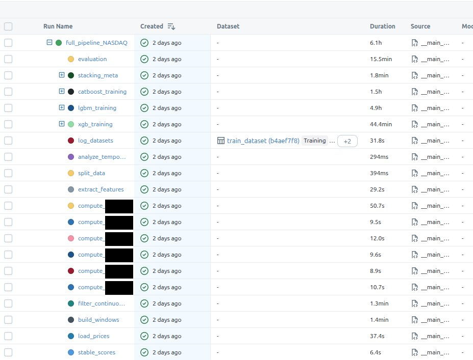
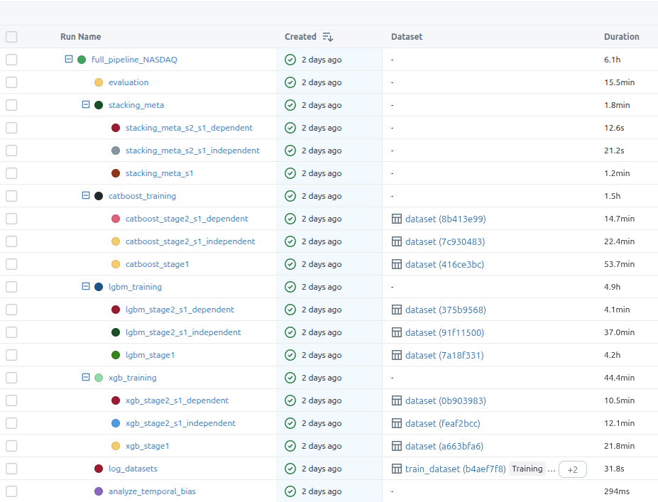
The first image shows all the steps and the second one includes the model training substeps. There are two stages in the training, like I mentioned in the requirements section of this post, but what I didn’t mention there is that the second stage also has two branches. The dependent model trains on the outputs from s1 model and the independent one, well, it’s independent so it trains on the same data that’s used by s1 training, but it optimizes for a different metric.
After all base models are trained, I’m also training some stacking meta-models that are supposed to further improve the initial predictions.
Now the main training function:
async def train_full_pipeline(
        exchange: str,
        months_of_data: int,
        val_months: int = 12,
        test_months: int = 12,
        n_trials_s1: int = 350,
        n_trials_s2: int = 350,
        data_to: date | None = None,
) -> PipelineResult:
    run_name = f"full_pipeline_{exchange}"

    with mlflow.start_run(run_name=run_name) as run:
        mlflow.log_params(dict(
            months_of_data=months_of_data,
            val_months=val_months,
            test_months=test_months,
            n_trials_s1=n_trials_s1,
            n_trials_s2=n_trials_s2,
            exchange=exchange,
        ))
        if data_to is not None:
            mlflow.log_param("data_to", str(data_to))

        trained_models, df_test = await _train_models_only(
            months_of_data=months_of_data,
            val_months=val_months,
            test_months=test_months,
            n_trials_s1=n_trials_s1,
            n_trials_s2=n_trials_s2,
            exchange=exchange,
            parent_run_id=run.info.run_id,
            data_to=data_to,
        )

        with mlflow.start_run(run_name="evaluation", nested=True):
            all_evaluations = evaluate_models_on_data(trained_models, df_test)
            best = select_best_pipeline(all_evaluations)

            _log_evaluation_to_mlflow(all_evaluations, best, trained_models)

    return PipelineResult(
        trained_models=trained_models,
        best_s1_mode=best.s1_mode,
        best_s2_mode=best.s2_mode,
        best_s2_training_mode=best.s2_training_mode,
        all_evaluations=all_evaluations,
        best_metrics=best.metrics,
        best_validation=best.validation,
    )
I think it’s rather cleanly written, but just for completeness, the most important parts are:
- start mlflow run under which all will be put
- train the models
- run evaluation
- evaluate the models on test data
- save the best models (which I’m calling pipeline here)
async def _train_models_only(
    months_of_data: int,
    val_months: int,
    test_months: int,
    n_trials_s1: int,
    n_trials_s2: int,
    exchange: str | None,
    parent_run_id: str | None = None,
    data_to: date | None = None,
) -> tuple[TrainedModels, pd.DataFrame]:
    data: PreparedData = await prepare_data(
        months_of_data=months_of_data,
        val_months=val_months,
        test_months=test_months,
        exchange=exchange,
        data_to=data_to,
    )
    trained_models = await _train_on_prepared_data(
        data=data,
        exchange=exchange,
        n_trials_s1=n_trials_s1,
        n_trials_s2=n_trials_s2,
        parent_run_id=parent_run_id,
    )

    return trained_models, data.df_test
The prepare_data function is very lengthy and has a lot of details strictly related to what I’m NOT trying to include in this post, so I’ll omit it. The only important detail is its return type:
class PreparedData(NamedTuple):
    df_train: pd.DataFrame
    df_val: pd.DataFrame
    df_test: pd.DataFrame
    daily_stock_data: pd.DataFrame
As for the other function:
async def _train_on_prepared_data(
    data: PreparedData,
    exchange: str | None,
    n_trials_s1: int,
    n_trials_s2: int,
    parent_run_id: str | None = None,
) -> TrainedModels:
    exchange_for_registry = exchange or "combined"

    # Train XGBoost first (uses GPU)
    xgb_result = await asyncio.to_thread(
        train_xgb_models,
        df_train=data.df_train,
        df_val=data.df_val,
        exchange=exchange_for_registry,
        n_trials_s1=n_trials_s1,
        n_trials_s2=n_trials_s2,
        parent_run_id=parent_run_id,
    )

    # Then train CatBoost (GPU) and LGBM (CPU) in parallel - no GPU memory conflict
    lgbm_result, catboost_result = await asyncio.gather(
        asyncio.to_thread(
            train_lgbm_models,
            df_train=data.df_train,
            df_val=data.df_val,
            exchange=exchange_for_registry,
            n_trials_s1=n_trials_s1,
            n_trials_s2=n_trials_s2,
            parent_run_id=parent_run_id,
        ),
        asyncio.to_thread(
            train_catboost_models,
            df_train=data.df_train,
            df_val=data.df_val,
            exchange=exchange_for_registry,
            n_trials_s1=n_trials_s1,
            n_trials_s2=n_trials_s2,
            parent_run_id=parent_run_id,
        ),
    )

    # Train stacking meta-models
    stacking_result = _train_stacking_meta_models(
        df_train=data.df_train,
        df_val=data.df_val,
        xgb_result=xgb_result,
        lgbm_result=lgbm_result,
        catboost_result=catboost_result,
        exchange=exchange_for_registry,
        parent_run_id=parent_run_id,
    )

    return TrainedModels(
        xgb_model_s1=xgb_result.s1_model,
        xgb_model_s2_s1_independent=xgb_result.s2_model_s1_independent,
        xgb_model_s2_s1_dependent=xgb_result.s2_model_s1_dependent,
        lgbm_model_s1=lgbm_result.s1_model,
        lgbm_model_s2_s1_independent=lgbm_result.s2_model_s1_independent,
        lgbm_model_s2_s1_dependent=lgbm_result.s2_model_s1_dependent,
        catboost_model_s1=catboost_result.s1_model,
        catboost_model_s2_s1_independent=catboost_result.s2_model_s1_independent,
        catboost_model_s2_s1_dependent=catboost_result.s2_model_s1_dependent,
        xgb_features_s1=xgb_result.s1_features,
        xgb_features_s2_s1_independent=xgb_result.s2_features_s1_independent,
        xgb_features_s2_s1_dependent=xgb_result.s2_features_s1_dependent,
        lgbm_features_s1=lgbm_result.s1_features,
        lgbm_features_s2_s1_independent=lgbm_result.s2_features_s1_independent,
        lgbm_features_s2_s1_dependent=lgbm_result.s2_features_s1_dependent,
        catboost_features_s1=catboost_result.s1_features,
        catboost_features_s2_s1_independent=catboost_result.s2_features_s1_independent,
        catboost_features_s2_s1_dependent=catboost_result.s2_features_s1_dependent,
        exchange=exchange,
        stacking_meta_s1=stacking_result.meta_s1,
        stacking_meta_s2_s1_independent=stacking_result.meta_s2_indep,
        stacking_meta_s2_s1_dependent=stacking_result.meta_s2_dep,
        stacking_meta_s1_info=stacking_result.meta_s1_info,
        stacking_meta_s2_s1_independent_info=stacking_result.meta_s2_indep_info,
        stacking_meta_s2_s1_dependent_info=stacking_result.meta_s2_dep_info,
    )
To my surprise CatBoost-GPU training was eating up almost all of my 16GB GPU-RAM and it was causing out of memory exceptions with XGBoost being trained in parallel (or the presence of XGB OOM-ed CatBoost, it doesn’t matter). It didn’t happen always, but often enough for me to address it on the architectural level expressed in this function. It first trains XGB, and then starts parallel training of CatBoost and LightGBM. It’s fine to use .to_thread + await, because 99% of the processing time for all three models will be spent in the C++ code, outside normal python, so it won’t block Python’s main thread. And why am I even using async code? Well, because I implemented my training pipeline inside FastAPI’s background jobs system.
I won’t show you all three train_*_models, because they basically look the same. Let’s focus on the one that trains XGB:
class XGBTrainingResult(NamedTuple):
    s1_model: xgb.XGBClassifier
    s2_model_s1_independent: xgb.XGBClassifier
    s2_model_s1_dependent: xgb.XGBClassifier
    s1_features: list[str]
    s2_features_s1_independent: list[str]
    s2_features_s1_dependent: list[str]
    s1_params: dict
    s2_params_s1_independent: dict
    s2_params_s1_dependent: dict


def train_xgb_models(
    df_train: pd.DataFrame,
    df_val: pd.DataFrame,
    exchange: str,
    n_trials_s1: int = N_TRIALS_S1,
    n_trials_s2: int = N_TRIALS_S2,
    parent_run_id: str | None = None,
) -> XGBTrainingResult:
    with mlflow.start_run(run_name="xgb_training", nested=parent_run_id is None):
        if parent_run_id:
            mlflow.set_tag("mlflow.parentRunId", parent_run_id)

        with mlflow.start_run(run_name="xgb_stage1", nested=True):
            s1_model, s1_features, s1_params = train_xgb_stage1(df_train, df_val, n_trials_s1)
            X_val_s1 = df_val[s1_features].astype("float64")
            signature = infer_signature(X_val_s1, s1_model.predict(X_val_s1.values))
            model_info = mlflow.xgboost.log_model(
                s1_model,
                name="xgb_s1_model",
                signature=signature,
                registered_model_name=f"xgb_s1_{exchange}",
            )
            eval_data = pd.DataFrame(X_val_s1, columns=s1_features)
            eval_data["label"] = df_val["is_big_move"].values

            mlflow.models.evaluate(
                model_info.model_uri,
                eval_data,
                targets="label",
                model_type="classifier",
            )

        df_val_s1_predictions = s1_model.predict(df_val[s1_features].values)

        with mlflow.start_run(run_name="xgb_stage2_s1_independent", nested=True):
            s2_model_indep, s2_features_indep, s2_params_indep = train_xgb_stage2_s1_independent(
                df_train, df_val, n_trials_s2
            )
            df_val_s2 = df_val.copy()
            df_val_s2["s1_pred"] = df_val_s1_predictions
            df_val_s2_filtered = df_val_s2[(df_val_s2["s1_pred"] == 1) & (df_val_s2["is_big_move"] == 1)]
            X_val_s2 = df_val_s2_filtered[s2_features_indep].astype("float64")
            signature = infer_signature(X_val_s2, s2_model_indep.predict(X_val_s2.values))
            model_info = mlflow.xgboost.log_model(
                s2_model_indep,
                name="xgb_s2_s1_independent_model",
                signature=signature,
                registered_model_name=f"xgb_s2_independent_{exchange}",
            )
            eval_data = pd.DataFrame(X_val_s2, columns=s2_features_indep)
            eval_data["label"] = df_val_s2_filtered["is_up"].values

            mlflow.models.evaluate(
                model_info.model_uri,
                eval_data,
                targets="label",
                model_type="classifier",
                extra_metrics=[precision_down_metric],
            )

        with mlflow.start_run(run_name="xgb_stage2_s1_dependent", nested=True):
            s2_model_dep, s2_features_dep, s2_params_dep = train_xgb_stage2_s1_dependent(
                df_train, df_val, s1_model, s1_features, n_trials_s2
            )
            df_val_s2_dep = df_val[df_val_s1_predictions == 1].copy()
            if len(df_val_s2_dep) > 0:
                X_val_s2_dep = df_val_s2_dep[s2_features_dep].astype("float64")
                signature = infer_signature(X_val_s2_dep, s2_model_dep.predict(X_val_s2_dep.values))
                model_info = mlflow.xgboost.log_model(
                    s2_model_dep,
                    name="xgb_s2_s1_dependent_model",
                    signature=signature,
                    registered_model_name=f"xgb_s2_dependent_{exchange}",
                )
                eval_data = pd.DataFrame(X_val_s2_dep, columns=s2_features_dep)
                eval_data["label"] = df_val_s2_dep["is_up"].values

                mlflow.models.evaluate(
                    model_info.model_uri,
                    eval_data,
                    targets="label",
                    model_type="classifier",
                    extra_metrics=[precision_down_metric],
                )

    return XGBTrainingResult(
        s1_model=s1_model,
        s2_model_s1_independent=s2_model_indep,
        s2_model_s1_dependent=s2_model_dep,
        s1_features=s1_features,
        s2_features_s1_independent=s2_features_indep,
        s2_features_s1_dependent=s2_features_dep,
        s1_params=s1_params,
        s2_params_s1_independent=s2_params_indep,
        s2_params_s1_dependent=s2_params_dep,
    )
The overall structure is:
- train stage 1 model (the one that focuses on recall)
- train stage 2 model that doesn’t depend on stage 1 outputs
- train stage 2 model that depends on stage 1 outputs
- log/register/evaluate models using mlflow function calls
Down the rabbit hole we go, let’s take a look at the final training functions:
Side note: I need to censor my code, because otherwise you’d see the PI information I’m trying to keep away from public eye :)
def get_selected_features(trial: optuna.Trial, groups: dict, min_groups: int = 2) -> list[str]:
    """Select feature groups using Optuna trial suggestions."""
    group_names = list(groups.keys())
    selections = {}

    for group_name in group_names:
        selections[group_name] = trial.suggest_categorical(f"use_{group_name}", [True, False])

    selected_count = sum(selections.values())

    if selected_count < min_groups:
        raise optuna.TrialPruned()

    selected_features = []

    for group_name, is_selected in selections.items():
        if is_selected:
            selected_features.extend(groups[group_name])

    return selected_features


def train_xgb_stage1(
    df_train: pd.DataFrame,
    df_val: pd.DataFrame,
    n_trials: int = N_TRIALS_S1,
    wf_folds: int = DEFAULT_WF_FOLDS,
    wf_val_months: int = DEFAULT_WF_VAL_MONTHS,
) -> tuple[xgb.XGBClassifier, list[str], dict]:
    df_combined = pd.concat([df_train, df_val], ignore_index=True)
    wf_splits = create_walk_forward_splits(df_combined, n_folds=wf_folds, val_months=wf_val_months)

    def objective(trial):
        selected_features = get_selected_features(trial, FEATURE_GROUPS_S1_XGB)
        max_depth = trial.suggest_int("max_depth", 3, 12)
        grow_policy = trial.suggest_categorical("grow_policy", ["depthwise", "lossguide"])
        params = dict(max_depth=max_depth, grow_policy=grow_policy,
                      learning_rate=trial.suggest_float("learning_rate", 0.005, 0.3, log=True),
                      n_estimators=trial.suggest_int("n_estimators", 100, 600),
                      min_child_weight=trial.suggest_int("min_child_weight", 1, 15),
                      gamma=trial.suggest_float("gamma", 1e-8, 5.0, log=True),
                      subsample=trial.suggest_float("subsample", 0.5, 1.0),
                      colsample_bytree=trial.suggest_float("colsample_bytree", 0.5, 1.0),
                      colsample_bylevel=trial.suggest_float("colsample_bylevel", 0.5, 1.0),
                      reg_alpha=trial.suggest_float("reg_alpha", 1e-8, 10.0, log=True),
                      reg_lambda=trial.suggest_float("reg_lambda", 1e-8, 10.0, log=True),
                      max_delta_step=trial.suggest_int("max_delta_step", 0, 10), device="cuda", tree_method="hist",
                      random_state=42, n_jobs=-1)

        if grow_policy == "lossguide":
            params["max_leaves"] = trial.suggest_int("max_leaves", 8, 256)

        params["early_stopping_rounds"] = EARLY_STOPPING_ROUNDS
        fold_scores = []

        for fold in wf_splits:
            fold_train_balanced = balance_binary_classes(fold.df_train, "xxx")
            X_train = fold_train_balanced[selected_features].values
            y_train = fold_train_balanced["xxx"].values
            X_val = fold.df_val[selected_features].values
            y_val = fold.df_val["xxx"].values
            model = xgb.XGBClassifier(**params)

            model.fit(X_train, y_train, eval_set=[(X_val, y_val)], verbose=False)

            y_pred = model.predict(X_val)

            fold_scores.append(_compute_s1_fold_score(y_val, y_pred))

        return np.mean(fold_scores)

    study = optuna.create_study(
        direction="maximize",
        pruner=optuna.pruners.MedianPruner(n_startup_trials=30, n_warmup_steps=15),
        sampler=optuna.samplers.TPESampler(seed=42),
    )

    study.optimize(objective, n_trials=n_trials, show_progress_bar=False)

    best_params = study.best_trial.params
    feature_params = {k: v for k, v in best_params.items() if k.startswith("use_")}
    model_params = {k: v for k, v in best_params.items() if not k.startswith("use_")}
    best_features = []

    for group_name, features in FEATURE_GROUPS_S1_XGB.items():
        if feature_params.get(f"use_{group_name}", False):
            best_features.extend(features)

    if len(best_features) == 0:
        best_features = [f for group in FEATURE_GROUPS_S1_XGB.values() for f in group]

    model_params.update(dict(device="cuda", tree_method="hist", random_state=42, n_jobs=-1,
                             early_stopping_rounds=EARLY_STOPPING_ROUNDS))

    df_train_balanced = balance_binary_classes(df_train, "xxx")
    X_train = df_train_balanced[best_features].values
    y_train = df_train_balanced["xxx"].values
    X_eval = df_val[best_features].values
    y_eval = df_val["xxx"].values
    model = xgb.XGBClassifier(**model_params)

    model.fit(X_train, y_train, eval_set=[(X_eval, y_eval)], verbose=False)
    mlflow.log_metric("best_f1_score", study.best_trial.value)
    mlflow.log_metric("n_features", len(best_features))
    mlflow.log_param("features", best_features)

    return model, best_features, model_params
As you can see, I’m giving optuna a really rich search space that contains the hyperparameters, and features (I have around 50 features). Then I’m balancing the classes and kicking off the training. There’s also some pruning and early stopping in place to speed up the training and prevent the overfitting if the loss is not improving.
As for the sampler, I defaulted to the popular choice of picking the TPESampler. In my case GridSampler wouldn’t do any good, because the search space is too big, CmaEsSampler is good for continuous spaces which is not the case here, and GPSampler… Well, I could have used it, but it’s also slower than TPESampler. Briefly: it’s a class that uses bayesian optimization technique to gradually narrow down the search space to the most promising areas. This dude will explain it best.
I’m also using a custom loss function to better focus on the objective:
def _compute_s1_fold_score(y_val: np.ndarray, y_pred: np.ndarray) -> float:
    precision = precision_score(y_val, y_pred, pos_label=1, zero_division=0)
    recall = recall_score(y_val, y_pred, pos_label=1, zero_division=0)

    if precision < MIN_PRECISION_S1:
        return precision * 0.1

    score = f1_score(y_val, y_pred, pos_label=1, zero_division=0)

    if recall > MAX_RECALL_S1:
        penalty = (recall - MAX_RECALL_S1) / (1.0 - MAX_RECALL_S1)
        score *= (1.0 - penalty) ** 2

    return score
If you’ve been doing machine learning for some time, you may know the sklearn’s fbeta_score function. At first I was thinking about using it to move the weight towards recall, but it wasn’t entirely what I wanted, and what I wanted was to have something with nonlinear/thresholding characteristic. fbeta_score does this:
- β < 1 - it will favor precision
- β > 1 - it will favor recall
What my implementation does is something different. If precision is below 0.3, then it punishes the model heavily by returning 10% of the already small precision score. On the other hand if the recall is too high, it applies a little less harsh penalty onto the f1 score. This expresses the intent of obtaining a model that will work like a not very dense fish net - it’s ok to catch a lot of flotsam and jetsam if we also catch a lot of fish.
Stage 2 training functions are 95% the same. The only difference is that their target variable is a bit different (although related) from stage 1 training target variable. I’m also using a different loss function for them, and after many trials I noticed that some features are more often picked up by stage 2, so that training phase is now using a constrained set of features - no point in making the training too long by making optuna search through garbage, right?
Stacking methods
Before I explain stacking, I’ll tell you how I implemented result reconciliation/aggregation with the two-stage, three-model-per-stage approach: I used ensembling.
…and before that I’ll tell you what do I mean by that, I’ll just drop a bomb: ensembles didn’t always outperform single models. But they usually did :)
So, in my case ensembling meant… Actually just read the damned code:
# ENSEMBLE_AVG
# S1:
avg_proba = (xgb_s1_proba + lgbm_s1_proba + catboost_s1_proba) / 3
df_eval["s1_pred_xxx"] = (avg_proba > 0.5).astype(int)

# S2:
df_eval["s2_avg_proba"] = (xgb_proba + lgbm_proba + catboost_proba) / 3
df_eval["xxx"] = (s1_pred == 1) & (s2_avg_proba >= 0.5)
Intuition: the probability of the three models is averaged. If the mean is > 0.5 -> prediction == True. It’s a somewhat “democratic” way of voting on what the result will be returned as.
# ENSEMBLE_AND
# S1:
df_eval["s1_pred_xxx"] = (xgb_s1_pred & lgbm_s1_pred & catboost_s1_pred).astype(int)
df_eval["s1_pred_proba"] = np.minimum(np.minimum(xgb_proba, lgbm_proba), catboost_proba)

# S2:
df_eval["xxx"] = (s1_pred == 1) & (xgb_pred == 1) & (lgbm_pred == 1) & (catboost_pred == 1)
df_eval["s2_pred_proba"] = df_eval[["s2_xgb_proba", "s2_lgbm_proba", "s2_catboost_proba"]].min(axis=1)
Intuition: all models need to agree, and the probability is a minimum out of all three. It’s a more conservative approach that will generate a lower number of signals.
Ok, so it’s all cool, but can this be made better? Turns out it can - with stacking.
The problem with ENSEMBLE_AVG and ENSEMBLE_AND is that they treat all models equally. But what if XGBoost is consistently better at detecting certain patterns while CatBoost excels at others? What if LightGBM tends to be overconfident?
With simple averaging, you’re essentially saying: “I trust all three of you equally.” and that’s somewhat naive.
With stacking, instead of hardcoding how to combine predictions, you train another model (the”meta-model”) to learn the optimal combination:
# Step 1: Get probability predictions from all base models
meta_features = np.column_stack([
    xgb_proba,      # XGBoost's confidence
    lgbm_proba,     # LightGBM's confidence
    catboost_proba  # CatBoost's confidence
])

# Step 2: Train a meta-model on these "meta-features"
meta_model.fit(meta_features, actual_labels)

# Step 3: At inference time
final_prediction = meta_model.predict(meta_features)
The meta-model can learn things like:
- “When XGBoost says 0.9 but the other two say 0.3, trust XGBoost”
- “When all three hover around 0.5-0.6, it’s probably noise - predict 0”
- “CatBoost’s 0.7 is worth more than LightGBM’s 0.8”
In my implementation, I tried two meta-model types: Logistic Regression (essentially learned linear weights) and XGBoost (can capture non-linear interactions between base model predictions). The system picks whichever performs better on validation data.
One gotcha: you can’t train the meta-model on the same data the base models saw - they’d be overfit and the meta-model would learn to trust their memorization. That’s why I used out-of-fold (OOF) predictions: train base models on fold 1-4, predict on fold 5, repeat for all folds, then train meta-model on those “honest” predictions.
def _train_stacking_meta_models(
    df_train: pd.DataFrame,
    df_val: pd.DataFrame,
    xgb_result,
    lgbm_result,
    catboost_result,
    exchange: str,
    parent_run_id: str | None = None,
) -> StackingMetaModelsResult:
    with mlflow.start_run(run_name="stacking_meta", nested=True, parent_run_id=parent_run_id):
        mlflow.log_param("exchange", exchange)
        mlflow.log_param("meta_feature_names", META_FEATURE_NAMES)

        # Generate OOF predictions for S1
        with mlflow.start_run(run_name="stacking_meta_s1", nested=True):
            train_meta_s1, train_labels_s1, val_meta_s1, val_labels_s1 = generate_oof_predictions(
                df_train=df_train,
                df_val=df_val,
                xgb_model=xgb_result.s1_model,
                lgbm_model=lgbm_result.s1_model,
                catboost_model=catboost_result.s1_model,
                xgb_features=xgb_result.s1_features,
                lgbm_features=lgbm_result.s1_features,
                catboost_features=catboost_result.s1_features,
                target_col="xxx",
            )
            meta_s1_result = train_meta_model_s1(train_meta_s1, train_labels_s1, val_meta_s1, val_labels_s1)
            meta_s1_info = _log_meta_model_to_mlflow(meta_s1_result, val_meta_s1, "s1", exchange)
            meta_s1 = meta_s1_result.winner.meta_model

        df_train_s2 = df_train[df_train["xxx"] == 1].copy()
        df_val_s2 = df_val[df_val["xxx"] == 1].copy()

        # S2 Independent
        if len(df_train_s2) >= 50 and len(df_val_s2) >= 20:
            with mlflow.start_run(run_name="stacking_meta_s2_s1_independent", nested=True):
                train_meta_s2_indep, train_labels_s2_indep, val_meta_s2_indep, val_labels_s2_indep = generate_oof_predictions(
                    df_train=df_train_s2,
                    df_val=df_val_s2,
                    xgb_model=xgb_result.s2_model_s1_independent,
                    lgbm_model=lgbm_result.s2_model_s1_independent,
                    catboost_model=catboost_result.s2_model_s1_independent,
                    xgb_features=xgb_result.s2_features_s1_independent,
                    lgbm_features=lgbm_result.s2_features_s1_independent,
                    catboost_features=catboost_result.s2_features_s1_independent,
                    target_col="is_up",
                )
                meta_s2_indep_result = train_meta_model_s2(
                    train_meta_s2_indep, train_labels_s2_indep, val_meta_s2_indep, val_labels_s2_indep
                )
                meta_s2_indep_info = _log_meta_model_to_mlflow(
                    meta_s2_indep_result, val_meta_s2_indep, "s2_s1_independent", exchange
                )
                meta_s2_indep = meta_s2_indep_result.winner.meta_model
        else:
            meta_s2_indep = None
            meta_s2_indep_info = None
            mlflow.log_param("s2_s1_independent_skipped", True)
            mlflow.log_param("s2_s1_independent_skip_reason", f"train={len(df_train_s2)}, val={len(df_val_s2)}")

        # S2 Dependent
        train_s1_pred = xgb_result.s1_model.predict(df_train[xgb_result.s1_features].values)
        val_s1_pred = xgb_result.s1_model.predict(df_val[xgb_result.s1_features].values)
        df_train_s2_dep = df_train[train_s1_pred == 1].copy()
        df_val_s2_dep = df_val[val_s1_pred == 1].copy()

        if len(df_train_s2_dep) >= 50 and len(df_val_s2_dep) >= 20:
            with mlflow.start_run(run_name="stacking_meta_s2_s1_dependent", nested=True):
                train_meta_s2_dep, train_labels_s2_dep, val_meta_s2_dep, val_labels_s2_dep = generate_oof_predictions(
                    df_train=df_train_s2_dep,
                    df_val=df_val_s2_dep,
                    xgb_model=xgb_result.s2_model_s1_dependent,
                    lgbm_model=lgbm_result.s2_model_s1_dependent,
                    catboost_model=catboost_result.s2_model_s1_dependent,
                    xgb_features=xgb_result.s2_features_s1_dependent,
                    lgbm_features=lgbm_result.s2_features_s1_dependent,
                    catboost_features=catboost_result.s2_features_s1_dependent,
                    target_col="xxx",
                )
                meta_s2_dep_result = train_meta_model_s2(
                    train_meta_s2_dep, train_labels_s2_dep, val_meta_s2_dep, val_labels_s2_dep
                )
                meta_s2_dep_info = _log_meta_model_to_mlflow(
                    meta_s2_dep_result, val_meta_s2_dep, "s2_s1_dependent", exchange
                )
                meta_s2_dep = meta_s2_dep_result.winner.meta_model
        else:
            meta_s2_dep = None
            meta_s2_dep_info = None
            mlflow.log_param("s2_s1_dependent_skipped", True)
            mlflow.log_param("s2_s1_dependent_skip_reason", f"train={len(df_train_s2_dep)}, val={len(df_val_s2_dep)}")

    return StackingMetaModelsResult(
        meta_s1=meta_s1,
        meta_s2_indep=meta_s2_indep,
        meta_s2_dep=meta_s2_dep,
        meta_s1_info=meta_s1_info,
        meta_s2_indep_info=meta_s2_indep_info,
        meta_s2_dep_info=meta_s2_dep_info,
    )
That’s a lot of code, but it’s rather simple - it just trains meta models for each of the stages. What’s more interesting is the generate_oof_predictions function:
def generate_oof_predictions(
    df_train: pd.DataFrame,
    df_val: pd.DataFrame,
    xgb_model,
    lgbm_model,
    catboost_model,
    xgb_features: list[str],
    lgbm_features: list[str],
    catboost_features: list[str],
    target_col: str,
    n_folds: int = N_META_FOLDS,
) -> tuple[np.ndarray, np.ndarray, np.ndarray, np.ndarray]:
    y_train = df_train[target_col].values
    y_val = df_val[target_col].values
    n_train = len(df_train)
    xgb_oof = np.zeros(n_train)
    lgbm_oof = np.zeros(n_train)
    catboost_oof = np.zeros(n_train)
    skf = StratifiedKFold(n_splits=n_folds, shuffle=True, random_state=42)

    for fold_idx, (train_idx, val_idx) in enumerate(skf.split(df_train, y_train)):
        fold_train = df_train.iloc[train_idx]
        fold_val = df_train.iloc[val_idx]
        fold_train_balanced = balance_binary_classes(fold_train, target_col)
        fold_y_train_balanced = fold_train_balanced[target_col].values
        X_fold_train_xgb = fold_train_balanced[xgb_features].values
        X_fold_val_xgb = fold_val[xgb_features].values
        fold_xgb = xgb.XGBClassifier(
            **{k: v for k, v in xgb_model.get_params().items()
               if k not in ['early_stopping_rounds', 'callbacks']},
            early_stopping_rounds=30,
        )

        fold_xgb.fit(
            X_fold_train_xgb, fold_y_train_balanced,
            eval_set=[(X_fold_val_xgb, fold_val[target_col].values)],
            verbose=False,
        )

        xgb_oof[val_idx] = fold_xgb.predict_proba(X_fold_val_xgb)[:, 1]
        X_fold_train_lgbm = fold_train_balanced[lgbm_features].astype("float32")
        X_fold_val_lgbm = fold_val[lgbm_features].astype("float32")
        fold_lgbm = lgb.LGBMClassifier(
            **{k: v for k, v in lgbm_model.get_params().items() if k != 'callbacks'}
        )

        fold_lgbm.fit(
            X_fold_train_lgbm, fold_y_train_balanced,
            eval_set=[(X_fold_val_lgbm, fold_val[target_col].values)],
            callbacks=[lgb.early_stopping(30, verbose=False)],
        )

        lgbm_oof[val_idx] = fold_lgbm.predict_proba(X_fold_val_lgbm)[:, 1]

        X_fold_train_cb = fold_train_balanced[catboost_features].values
        X_fold_val_cb = fold_val[catboost_features].values
        cb_params = dict(catboost_model.get_params())

        cb_params.update(early_stopping_rounds=30, verbose=False, train_dir=None)

        fold_cb = CatBoostClassifier(**cb_params)

        fold_cb.fit(
            X_fold_train_cb, fold_y_train_balanced,
            eval_set=(X_fold_val_cb, fold_val[target_col].values),
        )

        catboost_oof[val_idx] = fold_cb.predict_proba(X_fold_val_cb)[:, 1]

    train_meta_features = create_meta_features(xgb_oof, lgbm_oof, catboost_oof)
    X_val_xgb = df_val[xgb_features].values
    X_val_lgbm = df_val[lgbm_features].astype("float32")
    X_val_cb = df_val[catboost_features].values
    xgb_val_proba = xgb_model.predict_proba(X_val_xgb)[:, 1]
    lgbm_val_proba = lgbm_model.predict_proba(X_val_lgbm)[:, 1]
    catboost_val_proba = catboost_model.predict_proba(X_val_cb)[:, 1]
    val_meta_features = create_meta_features(xgb_val_proba, lgbm_val_proba, catboost_val_proba)

    return train_meta_features, y_train, val_meta_features, y_val
The generate_oof_predictions function takes training data, validation data, and the three trained base models.
For training data, it splits into 5 folds. In each iteration, it trains fresh copies of all three models on 4 folds and predicts on the remaining fold. After 5 iterations, every training sample has a prediction from a model that never saw it.
For validation data, it just uses the original models directly - they never saw this data during training anyway, so no special treatment needed.
Finally, it combines the raw probabilities from all three models into “meta-features”: the three probabilities themselves, plus their mean, max, min, and an “agreement score” (what fraction of models said yes). Seven features total that the meta-model will learn from.
Evaluation
The last step in my pipeline evaluates all the trained models. Again, I won’t attach the full code, as it’s highly repetitive and boring. I’ll only show what’s the most important - a function that computes a result telling me if the given model pipeline gives me an edge in day trading:
def _compute_ranking_scores(evaluations: list["PipelineEvaluation"]) -> list["PipelineEvaluation"]:
    """
    Compute ranking-based scores for all pipeline evaluations.

    For each metric, pipelines are ranked and receive points based on position.
    Place 1 = N points, place N = 1 point (where N = number of pipelines).

    Modifiers:
    - 1st place in median return: +3 bonus points
    - Bias penalty: up to -BIAS_PENALTY_MULTIPLIER points for heavily skewed predictions
      (penalizes models that predict almost all up or almost all down)
    """
    valid_evals = [(i, e) for i, e in enumerate(evaluations) if "error" not in e.metrics]
    error_indices = {i for i, e in enumerate(evaluations) if "error" in e.metrics}

    if not valid_evals:
        return evaluations

    n = len(valid_evals)
    scores = {i: 0.0 for i, _ in valid_evals}
    ranking_metrics = [
        ("win_rate", True),
        ("precision", True),
        ("median_return", True),
        ("monthly_sharpe", True),
        ("confidence_return_corr", True),
        ("outlier_contribution", True),
        ("median_return_top10", True),
        ("precision_top10", True),
    ]
    median_return_ranks = {}

    for metric_name, higher_is_better in ranking_metrics:
        values = [(i, e.metrics.get(metric_name, 0)) for i, e in valid_evals]

        values.sort(key=lambda x: x[1], reverse=higher_is_better)

        for rank, (idx, _) in enumerate(values):
            points = n - rank
            scores[idx] += points

            if metric_name == "median_return":
                median_return_ranks[idx] = rank

    for idx, evaluation in valid_evals:
        if median_return_ranks.get(idx) == 0:
            scores[idx] += MEDIAN_RETURN_BONUS

    # Apply bias penalty only for extremely skewed predictions (< 20% or > 80%)
    for idx, evaluation in valid_evals:
        s2_up_ratio = evaluation.metrics.get("s2_up_ratio", 0.5)

        if s2_up_ratio < BIAS_PENALTY_THRESHOLD:
            # Penalty grows from 0 (at 20%) to BIAS_PENALTY_MULTIPLIER (at 0%)
            bias_penalty = (BIAS_PENALTY_THRESHOLD - s2_up_ratio) / BIAS_PENALTY_THRESHOLD * BIAS_PENALTY_MULTIPLIER
            scores[idx] -= bias_penalty
        elif s2_up_ratio > (1 - BIAS_PENALTY_THRESHOLD):
            # Penalty grows from 0 (at 80%) to BIAS_PENALTY_MULTIPLIER (at 100%)
            bias_penalty = (s2_up_ratio - (1 - BIAS_PENALTY_THRESHOLD)) / BIAS_PENALTY_THRESHOLD * BIAS_PENALTY_MULTIPLIER
            scores[idx] -= bias_penalty

    updated_evals = []

    for i, evaluation in enumerate(evaluations):
        if i in error_indices:
            new_score = -1.0
        else:
            new_score = scores[i]

        updated_evals.append(PipelineEvaluation(
            s1_mode=evaluation.s1_mode,
            s2_mode=evaluation.s2_mode,
            s2_training_mode=evaluation.s2_training_mode,
            metrics=evaluation.metrics,
            validation=evaluation.validation,
            score=new_score,
            has_edge=evaluation.has_edge,
        ))

    return updated_evals
I’ll unpack some of the ranking_metrics and wrap-up this lengthy post:
win_rate- this tells me how often the models are correct, on averagemonthly_sharpe- it’s a simplified version of the Sharpe ratio - high Sharpe means stable, predictable gains; low Sharpe means wild swings between monthsconfidence_return_corr- this one is actually the most important one as it informs me on the correlation between a model predicting with a high probability and actually observing the expected outcome
Summary
And that would be it! In 2025 I read a book about passive investing and the author said that speculative investing rarely beats passive investing, and if it does - it’s not stable. There are traders that can “beat the market” by 50% one year and loose all their money the next year. Well… He’s probably right, however, with the strategy I developed I’m hoping not to be one of the ones loosing all their money!